One-carat Blog: Chapter 3: Data manipulation using dplyr (part 2)

Continuation from the previous chapter

In the previous chapter we have seen quite a lot of functions from the dplyr package. In this chapter, we will see the rest of the functions where we learn how to handle row names, how to join columns and rows and different set operations in the dplyr package.

#loading neessary packages
library(dplyr)

rownames_to_column() & column_to_rownames()

Tidy data does not use row names. So use rownames_to_column() command to convert row names to a new column to the data. The function column_to_rownames() does the exact opposite of rownames_to_column() as it converts a column into rownames but make sure that the column you are converting into rownames does not contain NA values.

# mtcars dataset contains rownames
# creates new column called car_names which contains row names
mtcars %>% rownames_to_column(var = "car_names")

# returns the original mtcars dataset
mtcars %>% rownames_to_column(var = "car_names") %>%
  column_to_rownames(var = "car_names")

Combine tables/columns

bind_cols()

Joins columns with other columns. Similar function as that of cbind() from base R.

df1 <- tidytable::data.table(x = letters[1:5], y = c(1:5))
df2 <- tidytable::data.table(x = letters[3:7], y = c(6:10))
bind_cols(df1,df2)

#similar functionality
cbind(df1,df2)

bind_rows()

Joins rows with other rows. Similar function as that of rbind() from base R.

df1 <- tidytable::data.table(x = letters[1:5], y = c(1:5))
df2 <- tidytable::data.table(x = letters[3:7], y = c(6:10))
bind_rows(df1,df2)

#similar functionality
rbind(df1,df2)

The functions that are described below have the same functionality as that of bind_cols() but give you control over how the columns are joined.

Mutating joins and filtering joins

Mutating joins include left_join(), right_join(), inner_join() and full_join() and filtering joins include semi_join() and anti_join().

left_join()

In the code below, matching variables of df2 are joined with df1. In the final data, you can see that only kevin and sam from df2 are matched with df1, and only those row values are joined with df1. For those variables which didn’t get a match, the row values for those are filled with NA. You can interpret the variables with NA values as; both john and chris are not present in df2.

If you are familiar with set theory in mathematics, what we are doing essentially is similar to \((df1 \cap df2) \cup df1\).

df1 <- tidytable::data.table(x = c("john","kevin","chris","sam","sam"), y = 1:5)
df2 <- tidytable::data.table(x = c("kevin","sam", "bob"), z = 10:12)

df1 %>% left_join(df2)

right_join()

Similar to left_join() but here, you will be joining matching values from df1 to df2, the opposite of what we did earlier. As you can see only kevin and sam from the df1 is matched with df2, and only those row values are joined with df2. For the variables which didn’t get a match, the row values for those are filled with NA. You can interpret the variables with NA values as; bob is not present in df1.

This function, in the manner used here, is similar to \((df1 \cap df2) \cup df2\).

df1 <- tidytable::data.table(x = c("john","kevin","chris","sam","sam"), y = 1:5)
df2 <- tidytable::data.table(x = c("kevin","sam", "bob"), z = 10:12)

df1 %>% right_join(df2)

inner_join()

The function inner_join() compares both df1 and df2 variables and only joins rows with the same variables. Here only kevin and sam are common in both the dataframes so the row values of only those columns are joined and others are omitted.

This function is similar to \(df1 \cap df2\).

df1 <- tidytable::data.table(x = c("john","kevin","chris","sam","sam"), y = 1:5)
df2 <- tidytable::data.table(x = c("kevin","sam", "bob"), z = 10:12)

df1 %>% inner_join(df2)

full_join()

The function full_join() compares both df1 and df2 variables and joins all possible matches while retaining both mistakes in df1 and df2 with NA values.

This function is similar to \(df1 \cup df2\).

df1 <- tidytable::data.table(x = c("john","kevin","chris","sam","sam"), y = 1:5)
df2 <- tidytable::data.table(x = c("kevin","sam", "bob"), z = 10:12)

df1 %>% full_join(df2)

anti_join()

This is an example of filtering join. The function anti_join() compares df1 variables to and df2 variables and only outputs those variables of df1 which didn’t get a match with df2.

This function, in the manner used here, is similar to \(df1 \cap df2^c\).

df1 <- tidytable::data.table(x = c("john","kevin","chris","sam","sam"), y = 1:5)
df2 <- tidytable::data.table(x = c("kevin","sam", "bob"), z = 10:12)

df1 %>% anti_join(df2)

semi_join()

This is an example of filtering join. The function semi_join() is similar to inner_join() but it only gives variables of df1 which has a match with df2.

df1 <- tidytable::data.table(x = c("john","kevin","chris","sam","sam"), y = 1:5)
df2 <- tidytable::data.table(x = c("kevin","sam", "bob"), z = 10:12)

df1 %>% semi_join(df2)

Here is a nice graphical representation of the functions we just described now. Image source.

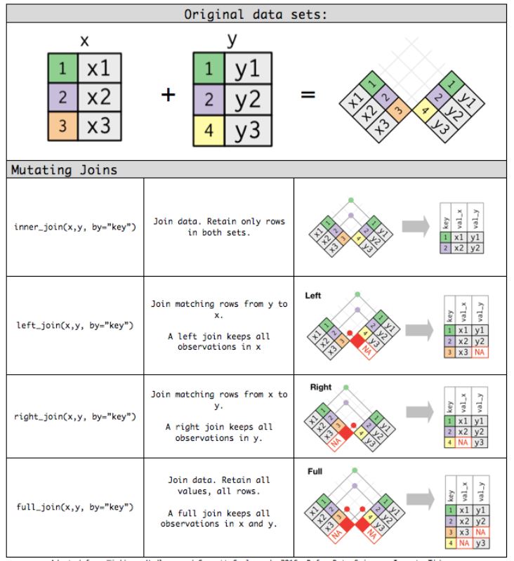
Figure 1: Source: RPubs.com

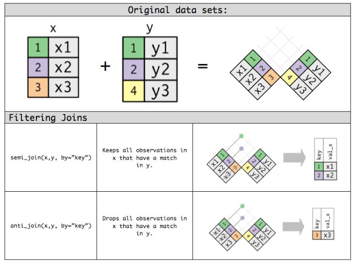
Figure 2: Source: RPubs.com

Additional commands for joins

Additionally, you can specify which common columns to match.

df1 <- tidytable::data.table(x = c("john","kevin","chris","sam","sam"), y = 1:5)
df2 <- tidytable::data.table(x = c("kevin","sam", "bob"), z = 10:12)

# match with column 'x'
df1 %>% left_join(df2, by = "x")

df3 <- tidytable::data.table(a = c("john","kevin","chris","sam","sam"), y = 1:5)
df4 <- tidytable::data.table(b = c("kevin","sam", "bob"), z = 10:12)

# matching with column having different names, a and b in this case
df3 %>% left_join(df4, by = c("a" = "b"))

Set operations

Similar to the mutating join functions that we had seen, there are different functions related to set theory operations.

intersect()

Outputs common rows in the dataset.

df1 <- tidytable::data.table(x = c("john","kevin","chris","sam","sam"))
df2 <- tidytable::data.table(x = c("kevin","sam", "bob"))

intersect(df1, df2)

       x
1: kevin
2:   sam

setdiff()

Outputs rows in first data frame but not in second data frame.

df1 <- tidytable::data.table(x = c("john","kevin","chris","sam","sam"))
df2 <- tidytable::data.table(x = c("kevin","sam", "bob"))

setdiff(df1, df2)

       x
1:  john
2: chris

union()

Outputs all the rows in both dataframes

df1 <- tidytable::data.table(x = c("john","kevin","chris","sam","sam"))
df2 <- tidytable::data.table(x = c("kevin","sam", "bob"))

union(df1, df2)

       x
1:  john
2: kevin
3: chris
4:   sam
5:   bob

setequal()

Checks whether two datasets have same number of rows.

df1 <- tidytable::data.table(x = c("john","kevin","chris","sam","sam"))
df2 <- tidytable::data.table(x = c("kevin","sam", "bob"))

setequal(df1, df2)

[1] FALSE

Summary

In this chapter, we have seen how to handle row names, how to combine columns and rows, what are mutating and filtering joins and various set operations. Thus to conclude this chapter, we have now learned almost all functions in the dplyr package and have seen how to manipulate data efficiently. With the knowledge of the pipe operator that we have seen in chapter 1, we are now equipped to write codes compactly and more clearly. I hope this chapter was useful for you and I will see you next time. Have a good day!

Previous chapter:
2: Data manipulation using dplyr (part 1)

References

Hadley Wickham, Romain François, Lionel Henry and Kirill Müller (2021). dplyr: A Grammar of Data Manipulation. R package version 1.0.7. https://CRAN.R-project.org/package=dplyr Here is the link to the cheat sheet explaining each function in dplyr.

Last updated on

[1] "2022-01-06 17:12:52 IST"

Chapter 3: Data manipulation using dplyr (part 2)