Introduction to dplyr package
The dplyr package is a grammar of data manipulation just like how ggplot2 is the grammar of data visualization. It helps us to apply a wide variety of functions such as;
- Summarising the dataset
- Applying selections and orderings as a function of a variable
- Creating new variables as a function of existing variables
We will see in-depth how to manipulate our data like a boss!
The pipe operator %>%
Perhaps the most amazing thing in making codes short and efficient is the pipe operator which is originally from the magrittr package which is made available for the dplyr package. The pipe operator helps you skip the intermediate steps of saving an object before you can use them in command. It does so by ‘piping’ together results from the first object to the function ahead of the pipe operator. The command x %>% y %>% z can be read as ‘take the result of x and use it with function y and take that result and use it with function z’. This is the gist of what the pipe operator does. Allow me to demonstrate.
library(ggplot2)
#dummy data
a <- c(sample(1:100, size = 50))
b <- c(sample(1:100, size = 50))
data <- as.data.frame(cbind(a,b))

#without %>%
data <- mutate(data, ab = a*b, twice_a = 2*a)
data_new <- filter(data, ab < 300, twice_a < 200)
ggplot(data_new, aes(ab, twice_a)) + geom_point()

#with %>%
data %>% mutate(ab = a*b, twice_a = 2*a) %>%
  filter(ab < 300, twice_a < 200) %>%
  ggplot(aes(ab, twice_a)) + geom_point()
As you can see, with pipe operator %>%, we did not have to save any objects in the intermediate steps and also it improved the overall clarity of the code. I have used a few commands from the dplyr package in the example given above. So without further ado let us delve into the dplyr package. For this chapter, I will be using the penguin dataset from the popular palmerpenguin package as an example.
#install palmerpenguins package
install.packages("palmerpenguins")
library(dplyr)
library(palmerpenguins)
Grouping the data
group_by()
The command group_by() allows us to group the data via existing variables. It allows for a ‘split-apply-combine’ way of getting output. First, it will split the data or group the data with the levels in the variable, then apply the function of our choice and then finally combine the results to give us a tabular output. On its own the command doesn’t do anything, we use it in conjunction with other commands to get results based on the grouping we specify. The command ungroup() is used to ungroup the data.
Summarising the data
summarise()
The summarise() command allows you to get the summary statistics of a variable or a column in the dataset. The result is given as tabular data. Many types of summary statistics can be obtained using the summarise() function. Some of them are given below. To calculate average values it is necessary to drop NA values from the dataset. Use drop_na() command from the tidyr package. The comments denote what each summary statistic is.
library(tidyr)
summary_data <- penguins %>% drop_na() %>%
  group_by(species) %>% # we are grouping/splitting the data according to species
  summarise(avg_mass = mean(body_mass_g), #mean mass
            median_mass = median(body_mass_g), #median mass
            max_mass = max(body_mass_g), #max value of mass, can also use min()
            standard_deviation_bill_length = sd(bill_length_mm), #standard deviation of bill_length
            sum_mass = sum(flipper_length_mm), #sum
            distinct_years = n_distinct(year), #distinct values in column year
            no_of_non_NAs = sum(!is.na(year)), #gives no of non NAs,
            length_rows = n(), #length of the rows
            iqr_mass = IQR(body_mass_g), #inter quartile range of mass
            median_absolute_deviation_mass = mad(body_mass_g), #median absolute deviation of mass
            variance_mass = var(body_mass_g)) # variance
#viewing summary as a table
paged_table(summary_data)
The number of non NA values will be the same as that of n() result as we have used drop_na()command in the beginning.
The base function summary() in R also gives the whole summary statistics of a dataset
summary(penguins) species island bill_length_mm bill_depth_mm
Adelie :152 Biscoe :168 Min. :32.10 Min. :13.10
Chinstrap: 68 Dream :124 1st Qu.:39.23 1st Qu.:15.60
Gentoo :124 Torgersen: 52 Median :44.45 Median :17.30
Mean :43.92 Mean :17.15
3rd Qu.:48.50 3rd Qu.:18.70
Max. :59.60 Max. :21.50
NA's :2 NA's :2
flipper_length_mm body_mass_g sex year
Min. :172.0 Min. :2700 female:165 Min. :2007
1st Qu.:190.0 1st Qu.:3550 male :168 1st Qu.:2007
Median :197.0 Median :4050 NA's : 11 Median :2008
Mean :200.9 Mean :4202 Mean :2008
3rd Qu.:213.0 3rd Qu.:4750 3rd Qu.:2009
Max. :231.0 Max. :6300 Max. :2009
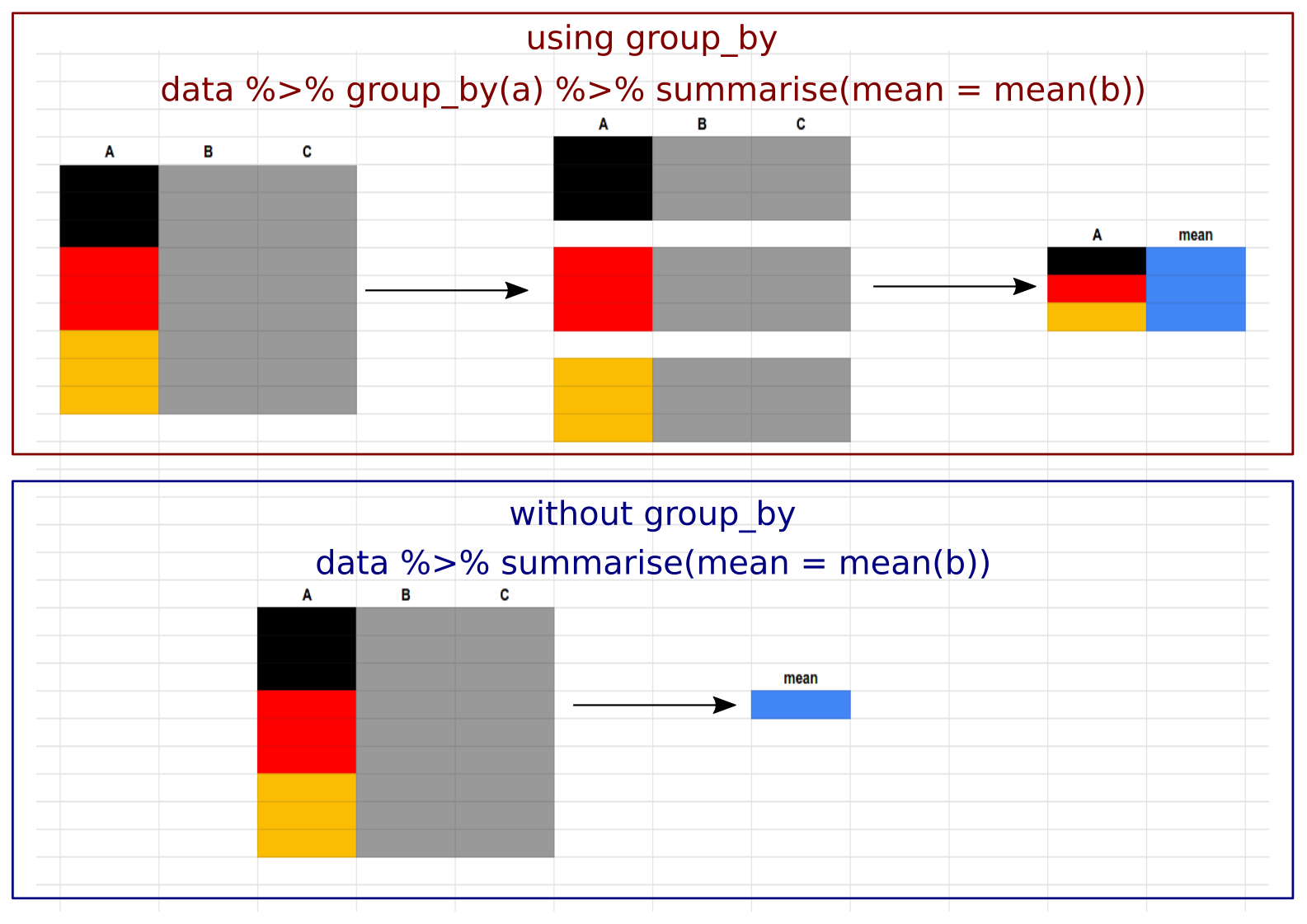
NA's :2 NA's :2 when to use group_by()
It can be confusing to decide when to use the group_by() function. In short, you should use it whenever you want any function to act separately on different groups present in the dataset. Here is a graphical representation of how the summarise() function is used to calculate the mean values of a dataset. When used with group_by() it calculates mean values for the respective groups in the data, but when group_by() is not used, it will calculate the mean value of the entire dataset irrespective of the different groups present and outputs a single column.
count()
The count() command is used to count the number of rows of a variable. Has the same function as that of n()
count <- penguins %>% group_by(species) %>%
  count(island)
#viewing count as a table
paged_table(count)
Manipulating cases or observations
The following functions affect rows to give a subset of rows in a new table as output.
filter()
Use filter() to filter rows corresponding to a given logical criteria
penguins %>% filter(body_mass_g < 3000)distinct()
Use distinct() to remove rows with duplicate or same values.
penguins %>% group_by(species) %>% distinct(body_mass_g)slice()
Use slice() to select rows by position.
penguins %>% slice(1:5) #slice from first row to fifth rowslice_sample()
Use slice_sample() to randomly select rows from the dataset. Instead of (n = ) you can also provide the proportion value (between 0 and 1) using (prop = ). For e.g. for a dataset with 10 rows, giving (prop = 0.5) will randomly sample 5 rows. Other related functions include;
preserve: Values includeTRUEto preserve grouping in a grouped dataset andFALSEto not preserve grouping while sampling.weight_by: Gives priority to a particular variable during sampling. An example is given below.replace: Values includeTRUEif you want sampling with replacement which can result in duplicate values,FALSEif you want sampling without replacement.
n = 4
#samples 4 rows randomly
penguins %>% slice_sample(n = 4)
weight_by
#sampling will favour rows with higher values of 'body_mass_g'
penguins %>% drop_na() %>% slice_sample(n = 4, weight_by = body_mass_g)
slice_min() and slice_max()
Use slice_min() to extract rows containing least values and use slice_max() to extract rows with greatest values. The function with_ties = FALSE is included to avoid tie values.
slice_min()
#first 4 rows containing least value in body mass
penguins %>% slice_min(body_mass_g, n = 4, with_ties = FALSE)
slice_max()
#first 4 rows containing least value in body mass
penguins %>% slice_max(body_mass_g, n = 4, with_ties = FALSE)
slice_head() and slice_tail()
Use slice_head() to extract first set of rows and use slice_tail() to extract last set of rows.
slice_head()
#samples first 4 rows
penguins %>% slice_head(n = 4)
slice_tail()
#samples last 4 rows
penguins %>% slice_tail(n = 4)
arrange()
Use arrange() to arrange rows in a particular order.
#arranging rows in descending order of bill length
#by default it arranges data by ascending order when no specifications are given
penguins %>% arrange(desc(bill_length_mm))
add_row()
Use add_row() to add rows to the dataset.
Name <- c("a", "b")
Age <- c(12,13)
data.frame(Name, Age) %>% add_row(Name = "c", Age = 15)
Manipulating variables or columns
The following functions affect columns to give a subset of columns in a new table as output.
pull()
Use pull() to extract columns as a vector, by name or index. Only the first 10 results are shown for easy viewing.
penguins %>% pull(body_mass_g) [1] 3750 3800 3250 NA 3450 3650 3625 4675 3475 4250
[ reached getOption("max.print") -- omitted 334 entries ]select()
Use select() to extract columns as tables, by name or index.
penguins %>% select(species, body_mass_g)relocate()
Use relocate() to move columns to new position. Results are not shown as these are trivial results.
#relocates 'species' column to last position
penguins %>% relocate(species, .after = last_col())
#relocates 'species' column before column 'year' and renames the column as 'penguins'
penguins %>% relocate(penguins = species, .before = year)#you can also relocate columns based on their class
#relocates all columns with 'character' class to last position
penguins %>% relocate(where(is.character), .after = last_col())rename()
Use rename() function to rename column names in the dataset.
#renames the column sex to gender
penguins %>% rename(gender = sex)
# A tibble: 344 × 8
species island bill_length_mm bill_depth_mm flipper_length_mm
<fct> <fct> <dbl> <dbl> <int>
1 Adelie Torgersen 39.1 18.7 181
2 Adelie Torgersen 39.5 17.4 186
3 Adelie Torgersen 40.3 18 195
4 Adelie Torgersen NA NA NA
5 Adelie Torgersen 36.7 19.3 193
6 Adelie Torgersen 39.3 20.6 190
7 Adelie Torgersen 38.9 17.8 181
8 Adelie Torgersen 39.2 19.6 195
9 Adelie Torgersen 34.1 18.1 193
10 Adelie Torgersen 42 20.2 190
# … with 334 more rows, and 3 more variables: body_mass_g <int>,
# gender <fct>, year <int>mutate()
Use mutate() function to create new columns or variables.
penguins %>% drop_na() %>%
  group_by(species) %>%
  mutate(mean_mass = mean(body_mass_g))
transmute()
Does the same function as mutate() but in the process will drop any other columns and give you a table with only the newly created columns.
penguins %>% drop_na() %>%
  group_by(species) %>%
  transmute(mean_mass = mean(body_mass_g))
across()
Use across() to summarise or mutate columns in the same way. First example shows across() used with summarise() function.
#summarise across columns body mass, bill length and bill depth
#and calculate the mean values
#since we are calculating mean values,
#NAs are dropped using 'drop_na() function from 'tidyr' package

penguins %>% drop_na() %>%
  group_by(species) %>%
  summarise(across(c(body_mass_g, bill_length_mm, bill_depth_mm), mean))
Second example showing across() used with mutate() function. We can efficiently create new columns using mutate() and across() together. Suppose we want to multiply all numerical values in a dataset with 2 and create new columns of those values. This can be done using the code below.
# define the function
two_times <- function(x) {
  2*x
}

# .name will rename the new columns with 'twice` prefix combined with existing col names
penguins %>% group_by(species) %>%
  mutate(across(where(is.numeric), two_times, .names = "two_times_{col}"))
The same code when used just with mutate() function will look like this
# define the function
two_times <- function(x) {
  2*x
}

#using only 'mutate()' function
penguins %>% group_by(species) %>%
  mutate(twice_bill_lenght = two_times(bill_length_mm),
         twice_body_mass = two_times(body_mass_g),
         .....)
So in this code, I will have to manually type all the col names and apply the operation individually which is too much of a hassle. Now we can better appreciate how efficient it is in using mutate() and across() functions together.
c_across()
The function c_across() is similar to the earlier mentioned across() function. But instead of doing a column-wise function, it applies function across columns in a row-wise manner. Now, most functions in R by default computes across columns, so to specify row-wise computation, we have to explicitly use the function rowwise() in conjunction with other functions. In the example below we will sum both bill and flipper lengths of the penguins in the penguins dataset and create a new column called ‘sum_of_lengths’
penguins %>% drop_na() %>%
  group_by(species) %>%
  rowwise() %>%
  transmute(sum_of_length = sum(c_across(c(bill_length_mm,flipper_length_mm))))
Summary
The dplyr package is the grammar of the data manipulation in R. It features well-made functions to help us summarise the data, group data by variables and manipulate columns and rows in the dataset. In this chapter, we learned in detail the different functions that help us manipulate data efficiently and have seen case examples also. In the next chapter, we will see the remaining set of functions in the dplyr package. See you!
Next chapter:
3. Data manipulation using dplyr (part 2) Previous chapter:
1. Data tidying using tidyr
References
Hadley Wickham, Romain François, Lionel Henry and Kirill Müller (2021). dplyr: A Grammar of Data Manipulation. R package version 1.0.7. https://CRAN.R-project.org/package=dplyr Here is the link to the cheat sheet explaining each function in
dplyr.Horst AM, Hill AP, Gorman KB (2020). palmerpenguins: Palmer Archipelago (Antarctica) penguin data. R package version 0.1.0. https://allisonhorst.github.io/palmerpenguins/
Hadley Wickham (2021). tidyr: Tidy Messy Data. R package version 1.1.4. https://CRAN.R-project.org/package=tidyr
Last updated on
[1] "2022-01-06 17:12:50 IST"