In this chapter, we will learn how to change the theme settings of a graph in ggplot2. The theme of a graph consists of non-data components present in your graph. This includes the different labels of the graph, fonts used, colour of axes, the background of the graph etc. By changing the theme we would not be changing or transforming how the data will look in the graph. Instead, we would only change the visual appearances in the graph and by doing so we can make it more aesthetically pleasing. Furthermore, we will see a few popular packages featuring ready to use themes. We will also learn about colour palettes and will see different packages associated with them.
Complete themes
The ggplot2 package features ready to use themes called ‘complete themes’. So before we begin customizing themes, let us plot a few graphs and see how these themes look like. For the plots, I have used the BirdNest dataset from the Stat2Data package in R. The BirdNest dataset contains nest and species characteristics of North American passerines. The data was collected by Amy R. Moore, as a student at Grinnell College in 1999.
- Getting the
BirdNestdataset and viewing how the dataset is structured.
install.packages("Stat2Data") #for installing Stat2Data package
install.packages("ggplot2") #for installing ggplot2 package

#load the packages
library(Stat2Data)
library(ggplot2)

data("BirdNest") #loading the BirdNest dataset
str(BirdNest) #for viewing structure of the dataset
So we have plenty of variables to play with. The tabs shown below are named according to the theme used in the plots. The description for each theme is taken from ggplot2 tidyverse webpage.
theme_gray()
theme_gray(): The signature ggplot2 theme with a grey background and white gridlines, designed to put the data forward yet make comparisons easy.
Show code
ggplot(BirdNest, aes(Nesttype, Length, fill = Nesttype)) + geom_boxplot() +
  labs(x= "Type of nest", y= "Mean body length for the species (in cm)",
       fill= "Nest type", title= "Relationship between body length and nest types",
       subtitle = "Data shown for 84 different species of North American passerines",
       caption= "DataSource: BridNest dataset in Stat2Data r-package") +
  theme_gray()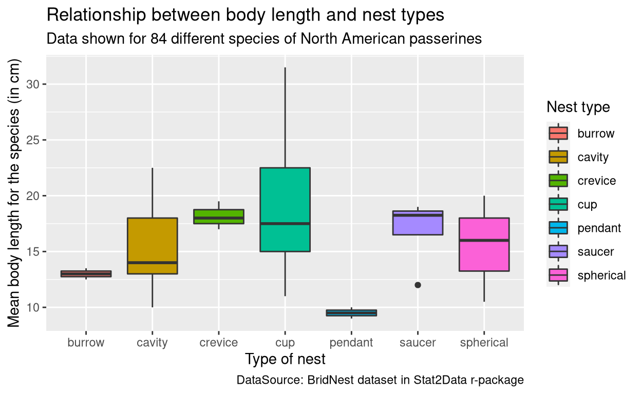
theme_bw()
theme_bw(): The classic dark-on-light ggplot2 theme. May work better for presentations displayed with a projector.
Show code
ggplot(BirdNest, aes(Nesttype, Length, fill = Nesttype)) + geom_boxplot() +
  labs(x= "Type of nest", y= "Mean body length for the species (in cm)",
       fill= "Nest type", title= "Relationship between body length and nest types",
       subtitle = "Data shown for 84 different species of North American passerines",
       caption= "DataSource: BridNest dataset in Stat2Data r-package") +
  theme_bw()
theme_linedraw()
theme_linedraw(): A theme with only black lines of various widths on white backgrounds, reminiscent of a line drawing. Serves a purpose similar to theme_bw(). Note that this theme has some very thin lines (<< 1 pt) which some journals may refuse.
Show code
ggplot(BirdNest, aes(Nesttype, Length, fill = Nesttype)) + geom_boxplot() +
  labs(x= "Type of nest", y= "Mean body length for the species (in cm)",
       fill= "Nest type", title= "Relationship between body length and nest types",
       subtitle = "Data shown for 84 different species of North American passerines",
       caption= "DataSource: BridNest dataset in Stat2Data r-package") +
  theme_linedraw()
theme_light()
theme_light(): A theme similar to theme_linedraw() but with light grey lines and axes, to direct more attention towards the data.
Show code
ggplot(BirdNest, aes(Nesttype, Length, fill = Nesttype)) + geom_boxplot() +
  labs(x= "Type of nest", y= "Mean body length for the species (in cm)",
       fill= "Nest type", title= "Relationship between body length and nest types",
       subtitle = "Data shown for 84 different species of North American passerines",
       caption= "DataSource: BridNest dataset in Stat2Data r-package") +
  theme_light()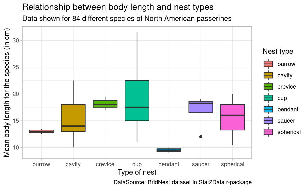
theme_dark()
theme_dark(): The dark cousin of theme_light(), with similar line sizes but a dark background. Useful to make thin coloured lines pop out.
Show code
ggplot(BirdNest, aes(Nesttype, Length, fill = Nesttype)) + geom_boxplot() +
  labs(x= "Type of nest", y= "Mean body length for the species (in cm)",
       fill= "Nest type", title= "Relationship between body length and nest types",
       subtitle = "Data shown for 84 different species of North American passerines",
       caption= "DataSource: BridNest dataset in Stat2Data r-package") +
  theme_dark()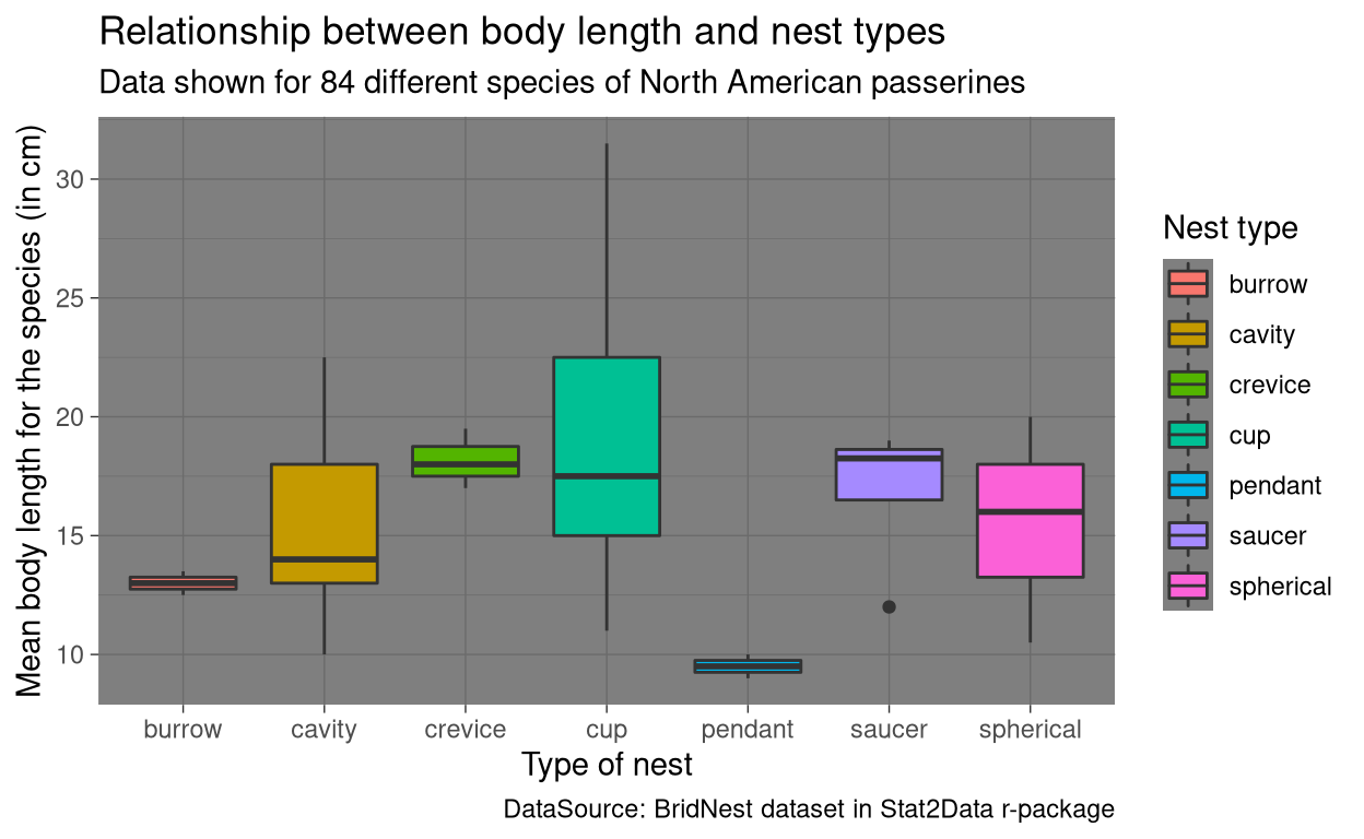
theme_minimal()
theme_minimal(): A minimalistic theme with no background annotations.
Show code
ggplot(BirdNest, aes(Nesttype, Length, fill = Nesttype)) + geom_boxplot() +
  labs(x= "Type of nest", y= "Mean body length for the species (in cm)",
       fill= "Nest type", title= "Relationship between body length and nest types",
       subtitle = "Data shown for 84 different species of North American passerines",
       caption= "DataSource: BridNest dataset in Stat2Data r-package") +
  theme_minimal()
theme_classic()
theme_classic(): A classic-looking theme, with x and y axis lines and no gridlines.
Show code
ggplot(BirdNest, aes(Nesttype, Length, fill = Nesttype)) + geom_boxplot() +
  labs(x= "Type of nest", y= "Mean body length for the species (in cm)",
       fill= "Nest type", title= "Relationship between body length and nest types",
       subtitle = "Data shown for 84 different species of North American passerines",
       caption= "DataSource: BridNest dataset in Stat2Data r-package") +
  theme_classic()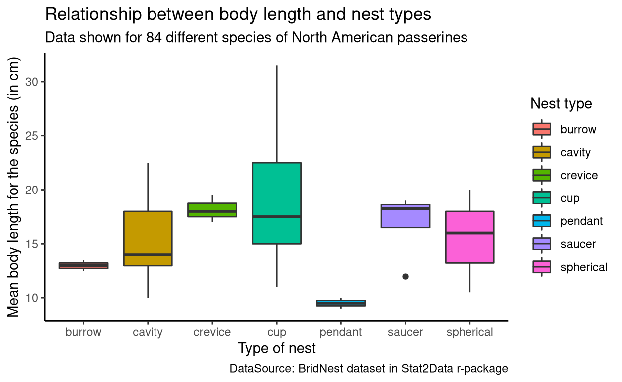
theme_void()
theme_void(): A completely empty theme.
Show code
ggplot(BirdNest, aes(Nesttype, Length, fill = Nesttype)) + geom_boxplot() +
  labs(x= "Type of nest", y= "Mean body length for the species (in cm)",
       fill= "Nest type", title= "Relationship between body length and nest types",
       subtitle = "Data shown for 84 different species of North American passerines",
       caption= "DataSource: BridNest dataset in Stat2Data r-package") +
  theme_void()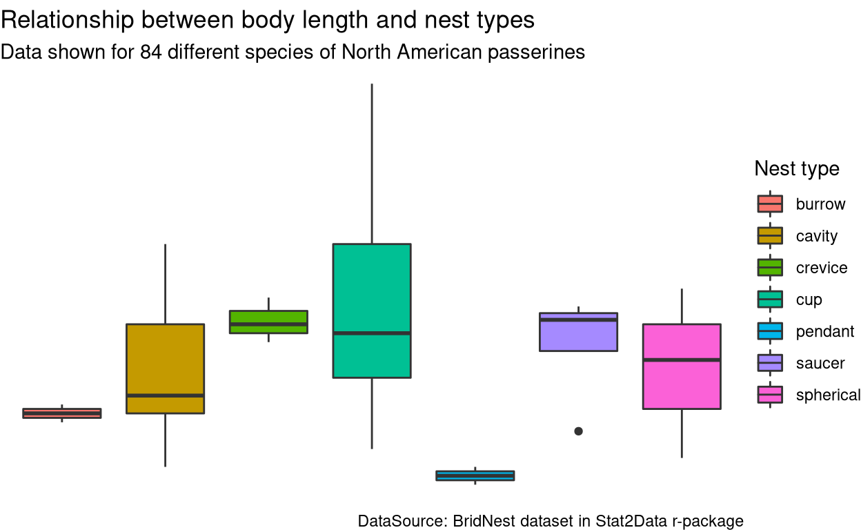
Themes from ggthemes package
If you want even more pre-built themes then you can try the ggthemes package. This package was developed by Dr. Jeffrey B. Arnold.
#install and load ggthemes package
install.packages("ggthemes")
library(ggthemes)
The tabs shown below are named after the themes present in ggthemes package. The description for each theme is taken from the ggthemes manual.
theme_base()
theme_base(): Theme similar to the default settings of the ‘base’ R graphics.
Show code
ggplot(BirdNest, aes(Nesttype, Length, fill = Nesttype)) + geom_boxplot() +
  labs(x= "Type of nest", y= "Mean body length for the species (in cm)",
       fill= "Nest type", title= "Relationship between body length and nest types",
       subtitle = "Data shown for 84 different species of North American passerines",
       caption= "DataSource: BridNest dataset in Stat2Data r-package") +
  theme_base() + theme(text = element_text(size = 10)) #size is reduced to accommodate the graph in the tab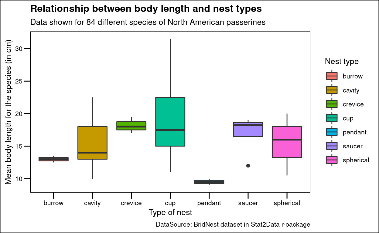
theme_calc()
theme_calc(): Theme similar to the default settings of LibreOffice Calc charts.
Show code
ggplot(BirdNest, aes(Nesttype, Length, fill = Nesttype)) + geom_boxplot() +
  labs(x= "Type of nest", y= "Mean body length for the species (in cm)",
       fill= "Nest type", title= "Relationship between body length and nest types",
       subtitle = "Data shown for 84 different species of North American passerines",
       caption= "DataSource: BridNest dataset in Stat2Data r-package") +
  theme_calc()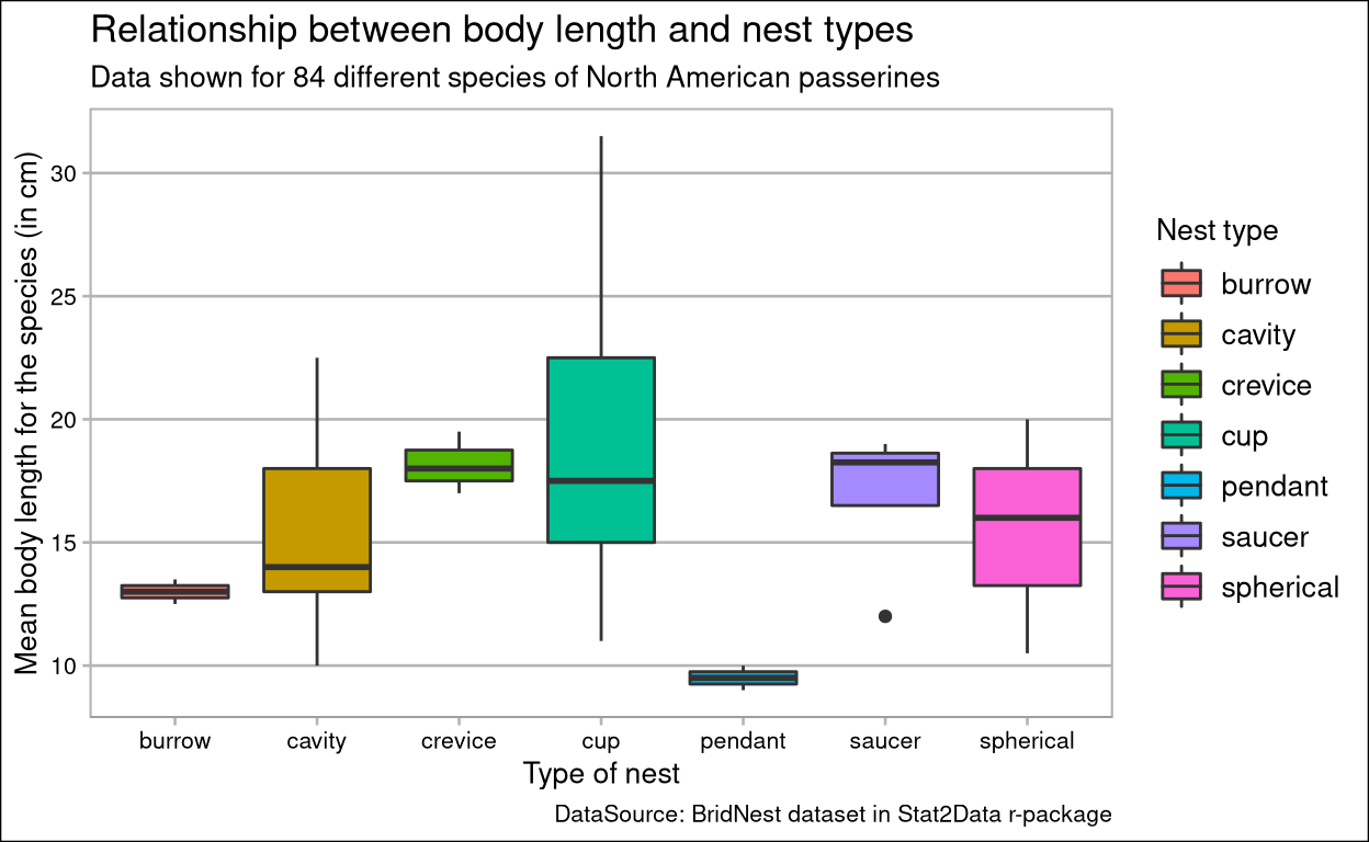
theme_clean()
theme_clean(): Clean ggplot theme with no panel background, black axis lines and grey fill colour for chart elements.
Show code
ggplot(BirdNest, aes(Nesttype, Length, fill = Nesttype)) + geom_boxplot() +
  labs(x= "Type of nest", y= "Mean body length for the species (in cm)",
       fill= "Nest type", title= "Relationship between body length and nest types",
       subtitle = "Data shown for 84 different species of North American passerines",
       caption= "DataSource: BridNest dataset in Stat2Data r-package") +
  theme_clean()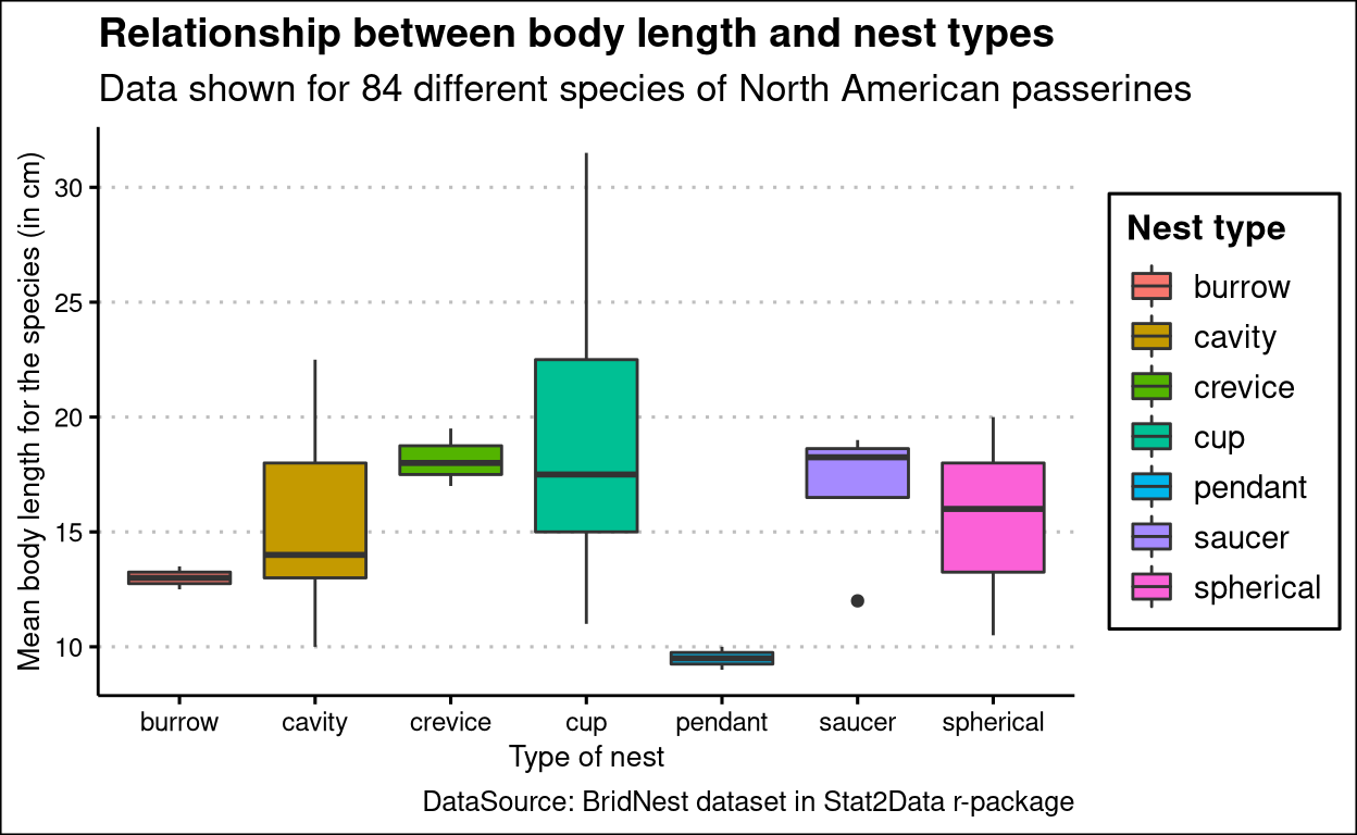
theme_economist()
theme_economist(): A theme that approximates the style of The Economist.
Show code
ggplot(BirdNest, aes(Nesttype, Length, fill = Nesttype)) + geom_boxplot() +
  labs(x= "Type of nest", y= "Mean body length for the species (in cm)",
       fill= "Nest type", title= "Relationship between body length and nest types",
       subtitle = "Data shown for 84 different species of North American passerines",
       caption= "DataSource: BridNest dataset in Stat2Data r-package") +
  theme_economist()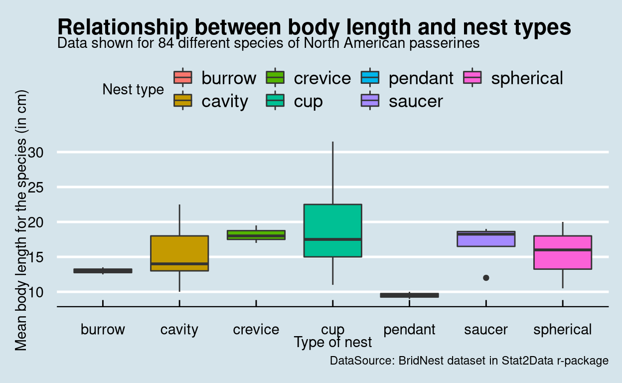
theme_excel()
theme_excel(): Theme to replicate the ugly monstrosity that was the old gray-background Excel chart. Please never use this. This theme should be combined with the
scale_colour_excel()color scale.
Show code
ggplot(BirdNest, aes(Nesttype, Length, fill = Nesttype)) + geom_boxplot() +
  labs(x= "Type of nest", y= "Mean body length for the species (in cm)",
       fill= "Nest type", title= "Relationship between body length and nest types",
       subtitle = "Data shown for 84 different species of North American passerines",
       caption= "DataSource: BridNest dataset in Stat2Data r-package") +
  theme_excel()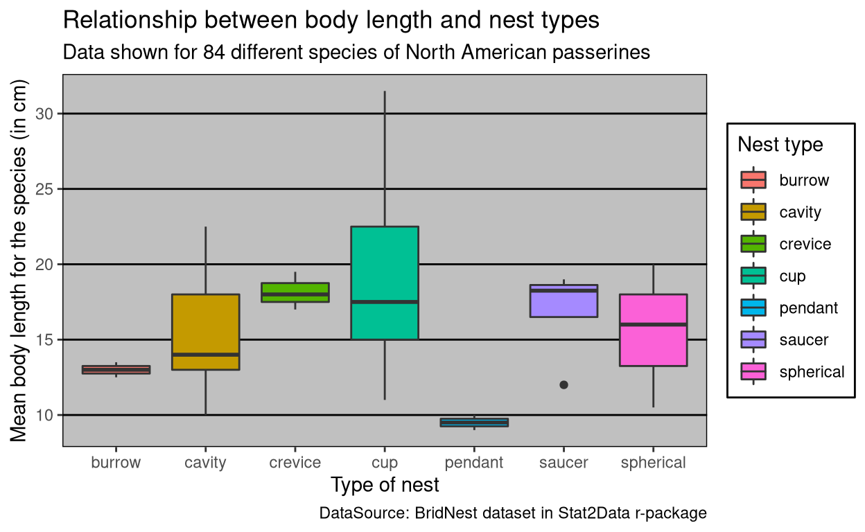
theme_excel_new()
theme_excel_new(): Theme for ggplot2 that is similar to the default style of charts in current versions of Microsoft Excel.
Show code
ggplot(BirdNest, aes(Nesttype, Length, fill = Nesttype)) + geom_boxplot() +
  labs(x= "Type of nest", y= "Mean body length for the species (in cm)",
       fill= "Nest type", title= "Relationship between body length and nest types",
       subtitle = "Data shown for 84 different species of North American passerines",
       caption= "DataSource: BridNest dataset in Stat2Data r-package") +
  theme_excel_new()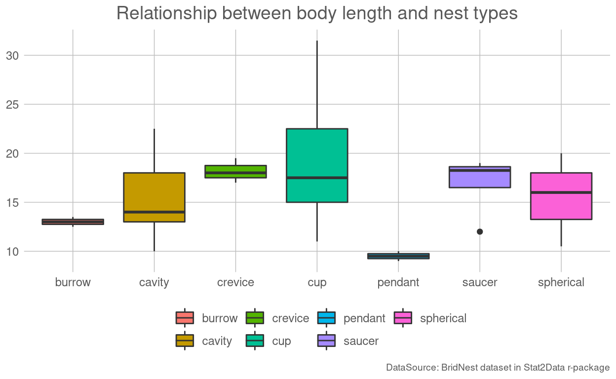
theme_few()
theme_few(): Theme based on the rules and examples from Stephen Few’s Show Me the Numbers and “Practical Rules for Using Color in Charts”.
Show code
ggplot(BirdNest, aes(Nesttype, Length, fill = Nesttype)) + geom_boxplot() +
  labs(x= "Type of nest", y= "Mean body length for the species (in cm)",
       fill= "Nest type", title= "Relationship between body length and nest types",
       subtitle = "Data shown for 84 different species of North American passerines",
       caption= "DataSource: BridNest dataset in Stat2Data r-package") +
  theme_few()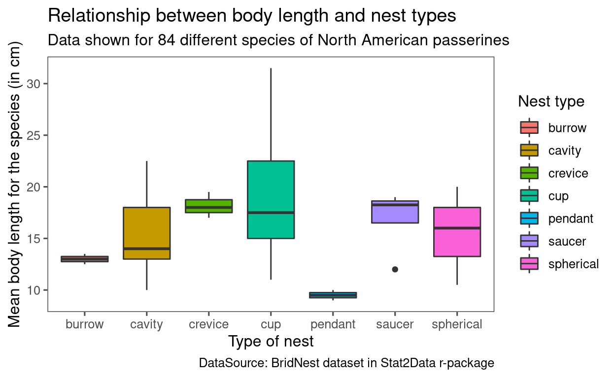
theme_fivethirtyeight()
theme_fivethirtyeight(): Theme inspired by the plots on FiveThirtyEight plots
Show code
ggplot(BirdNest, aes(Nesttype, Length, fill = Nesttype)) + geom_boxplot() +
  labs(x= "Type of nest", y= "Mean body length for the species (in cm)",
       fill= "Nest type", title= "Relationship between body length and nest types",
       subtitle = "Data shown for 84 different species of North American passerines",
       caption= "DataSource: BridNest dataset in Stat2Data r-package") +
  theme_fivethirtyeight()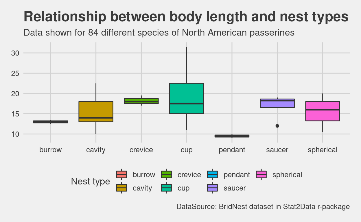
theme_foundation()
theme_foundation(): This theme is designed to be a foundation from which to build new themes, and not meant to be used directly.
theme_foundation()is a complete theme with only minimal number of elements defined. It is easier to create new themes by extending this one rather thantheme_gray()ortheme_bw(), because those themes define elements deep in the hierarchy.
Show code
ggplot(BirdNest, aes(Nesttype, Length, fill = Nesttype)) + geom_boxplot() +
  labs(x= "Type of nest", y= "Mean body length for the species (in cm)",
       fill= "Nest type", title= "Relationship between body length and nest types",
       subtitle = "Data shown for 84 different species of North American passerines",
       caption= "DataSource: BridNest dataset in Stat2Data r-package") +
  theme_foundation()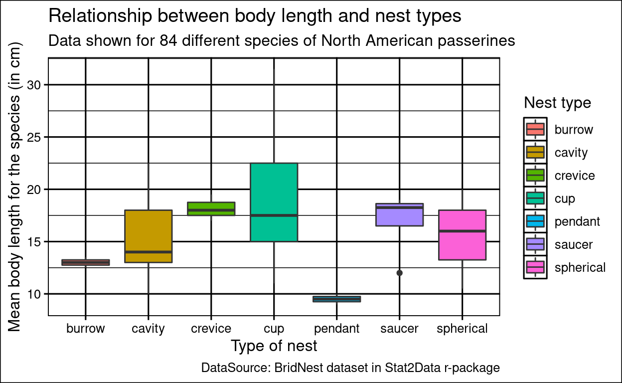
theme_gdocs()
theme_gdocs(): Theme similar to the default look of charts in Google Docs.
Show code
ggplot(BirdNest, aes(Nesttype, Length, fill = Nesttype)) + geom_boxplot() +
  labs(x= "Type of nest", y= "Mean body length for the species (in cm)",
       fill= "Nest type", title= "Relationship between body length and nest types",
       subtitle = "Data shown for 84 different species of North American passerines",
       caption= "DataSource: BridNest dataset in Stat2Data r-package") +
  theme_gdocs() + theme(text = element_text(size = 10)) #size is reduced to accommodate the graph in the tab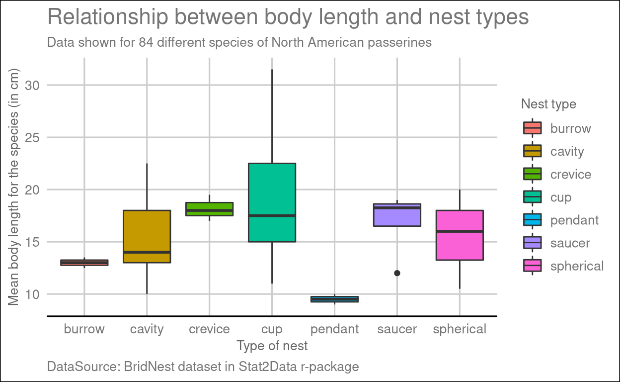
theme_hc()
theme_hc(): Theme based on Highcharts plots
Show code
ggplot(BirdNest, aes(Nesttype, Length, fill = Nesttype)) + geom_boxplot() +
  labs(x= "Type of nest", y= "Mean body length for the species (in cm)",
       fill= "Nest type", title= "Relationship between body length and nest types",
       subtitle = "Data shown for 84 different species of North American passerines",
       caption= "DataSource: BridNest dataset in Stat2Data r-package") +
  theme_hc()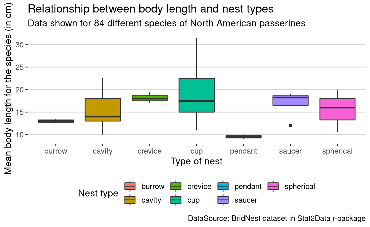
theme_igray()
theme_igray(): Theme with white panel and gray background.
Show code
ggplot(BirdNest, aes(Nesttype, Length, fill = Nesttype)) + geom_boxplot() +
  labs(x= "Type of nest", y= "Mean body length for the species (in cm)",
       fill= "Nest type", title= "Relationship between body length and nest types",
       subtitle = "Data shown for 84 different species of North American passerines",
       caption= "DataSource: BridNest dataset in Stat2Data r-package") +
  theme_igray()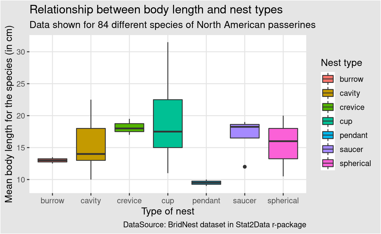
theme_map()
theme_map(): A clean theme that is good for displaying maps from
geom_map().
Show code
ggplot(BirdNest, aes(Nesttype, Length, fill = Nesttype)) + geom_boxplot() +
  labs(x= "Type of nest", y= "Mean body length for the species (in cm)",
       fill= "Nest type", title= "Relationship between body length and nest types",
       subtitle = "Data shown for 84 different species of North American passerines",
       caption= "DataSource: BridNest dataset in Stat2Data r-package") +
  theme_map()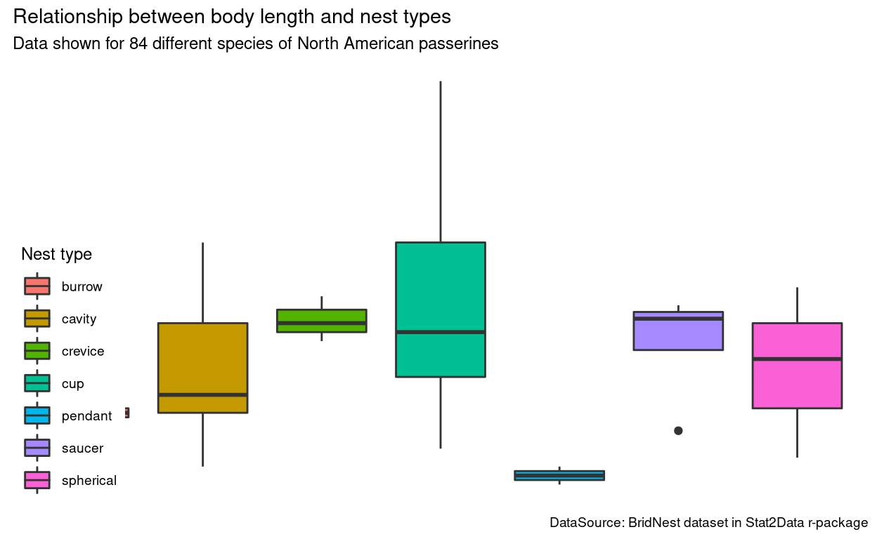
theme_pander()
theme_pander(): The pander ships with a default theme when the ’unify plots’ option is enabled via panderOptions, which is now also available outside of pander internals, like evals, eval.msgs or Pandoc.brew.
Show code
ggplot(BirdNest, aes(Nesttype, Length, fill = Nesttype)) + geom_boxplot() +
  labs(x= "Type of nest", y= "Mean body length for the species (in cm)",
       fill= "Nest type", title= "Relationship between body length and nest types",
       subtitle = "Data shown for 84 different species of North American passerines",
       caption= "DataSource: BridNest dataset in Stat2Data r-package") +
  theme_pander()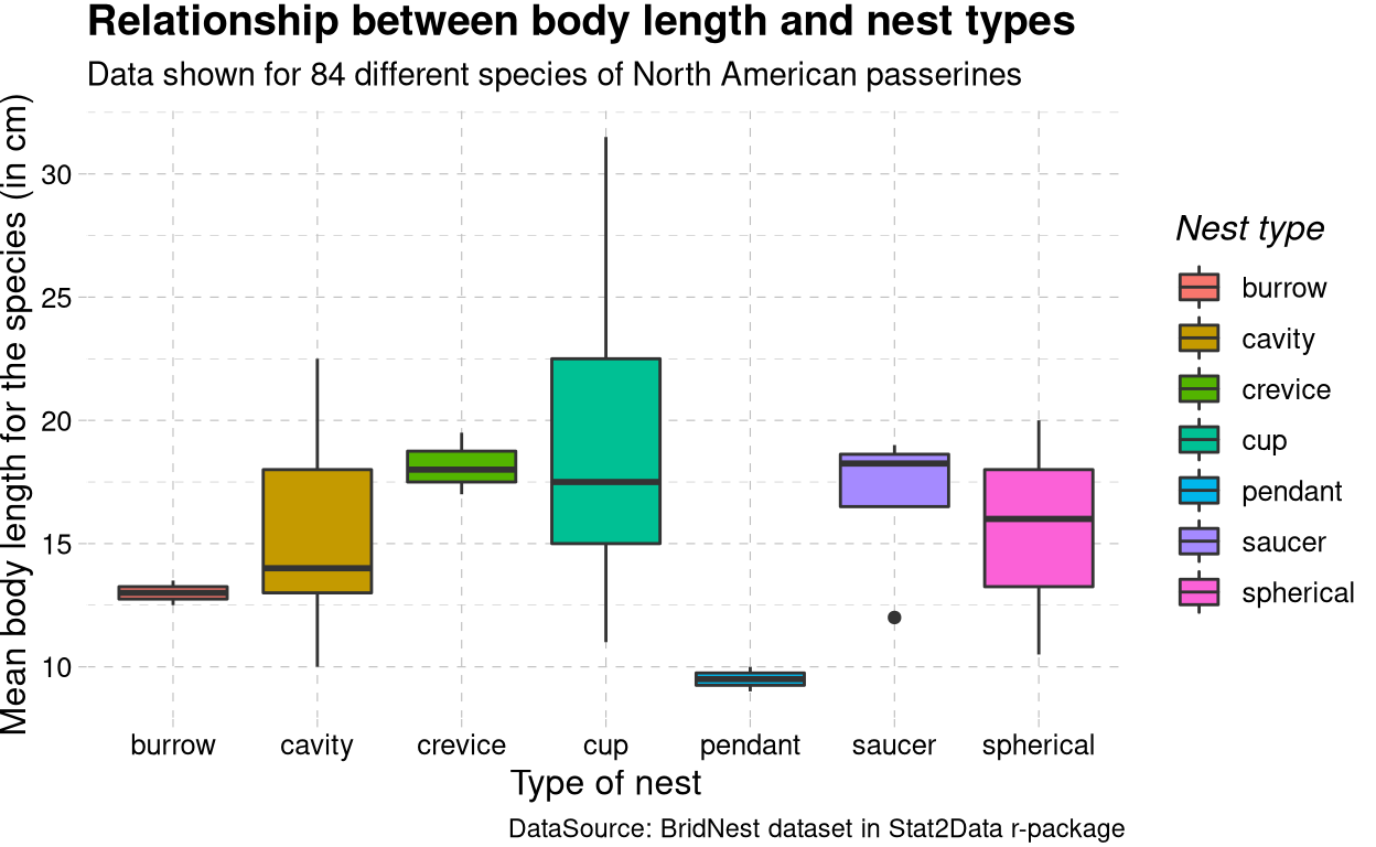
theme_par()
theme_par(): Theme which uses the current ‘base’ graphics parameter values from par(). Not all par() parameters, are supported, and not all are relevant to ggplot2 themes.
Show code
ggplot(BirdNest, aes(Nesttype, Length, fill = Nesttype)) + geom_boxplot() +
  labs(x= "Type of nest", y= "Mean body length for the species (in cm)",
       fill= "Nest type", title= "Relationship between body length and nest types",
       subtitle = "Data shown for 84 different species of North American passerines",
       caption= "DataSource: BridNest dataset in Stat2Data r-package") +
  theme_par() + theme(text = element_text(size = 9)) #size is reduced to accommodate the graph in the tab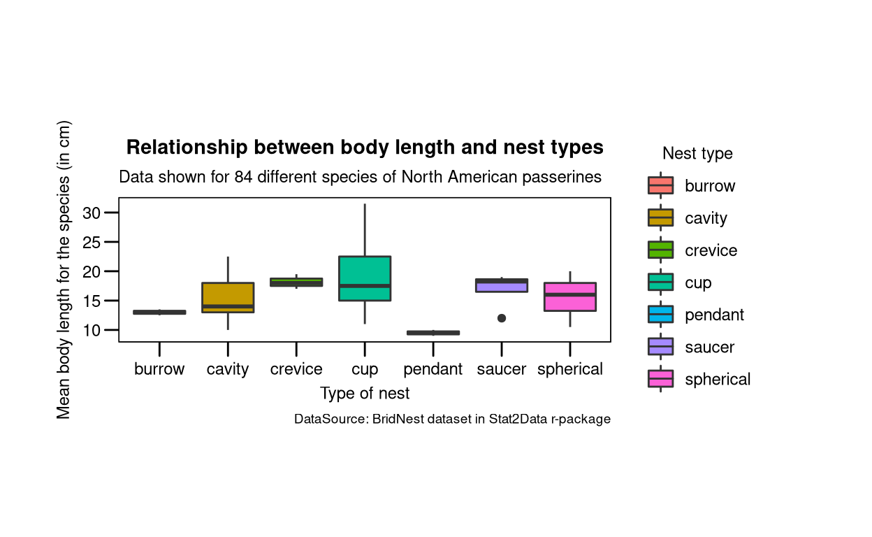
theme_solarized()
theme_solarized(): See https://ethanschoonover.com/solarized/ for a description of the Solarized palette.
Show code
ggplot(BirdNest, aes(Nesttype, Length, fill = Nesttype)) + geom_boxplot() +
  labs(x= "Type of nest", y= "Mean body length for the species (in cm)",
       fill= "Nest type", title= "Relationship between body length and nest types",
       subtitle = "Data shown for 84 different species of North American passerines",
       caption= "DataSource: BridNest dataset in Stat2Data r-package") +
  theme_solarized()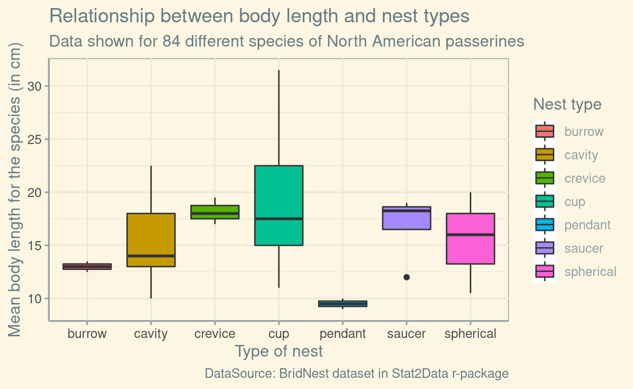
theme_solid()
theme_solid(): Theme with nothing other than a background color.
Show code
ggplot(BirdNest, aes(Nesttype, Length, fill = Nesttype)) + geom_boxplot() +
  labs(x= "Type of nest", y= "Mean body length for the species (in cm)",
       fill= "Nest type", title= "Relationship between body length and nest types",
       subtitle = "Data shown for 84 different species of North American passerines",
       caption= "DataSource: BridNest dataset in Stat2Data r-package") +
  theme_solid()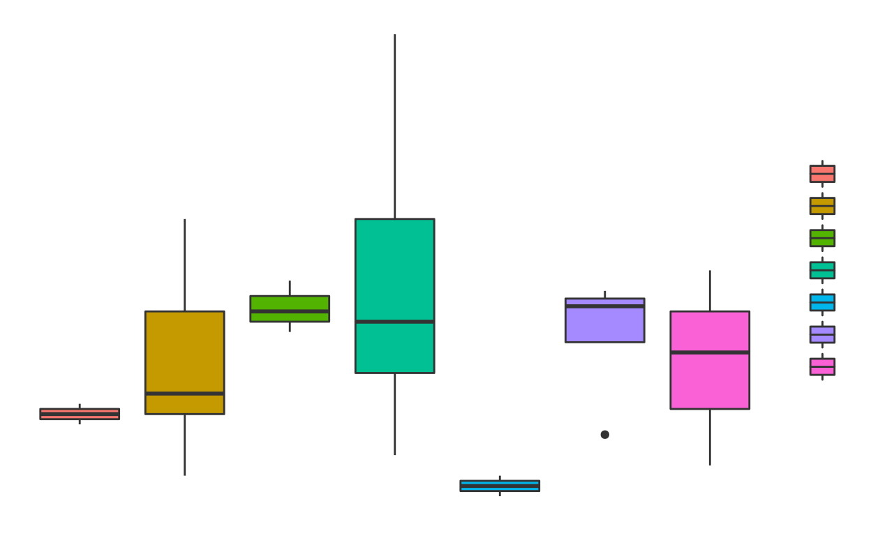
theme_stata()
theme_stata(): Themes based on Stata graph schemes.
Show code
ggplot(BirdNest, aes(Nesttype, Length, fill = Nesttype)) + geom_boxplot() +
  labs(x= "Type of nest", y= "Mean body length for the species (in cm)",
       fill= "Nest type", title= "Relationship between body length and nest types",
       subtitle = "Data shown for 84 different species of North American passerines",
       caption= "DataSource: BridNest dataset in Stat2Data r-package") +
  theme_stata()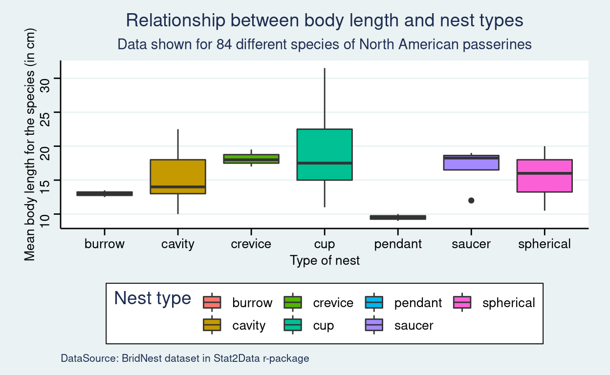
theme_tufte()
theme_tufte(): Theme based on Chapter 6 ’Data-Ink Maximization and Graphical Design’ of Edward Tufte The Visual Display of Quantitative Information. No border, no axis lines, no grids. This theme works best in combination with
geom_rug()orgeom_rangeframe().
Show code
ggplot(BirdNest, aes(Nesttype, Length, fill = Nesttype)) + geom_boxplot() +
  labs(x= "Type of nest", y= "Mean body length for the species (in cm)",
       fill= "Nest type", title= "Relationship between body length and nest types",
       subtitle = "Data shown for 84 different species of North American passerines",
       caption= "DataSource: BridNest dataset in Stat2Data r-package") +
  theme_tufte()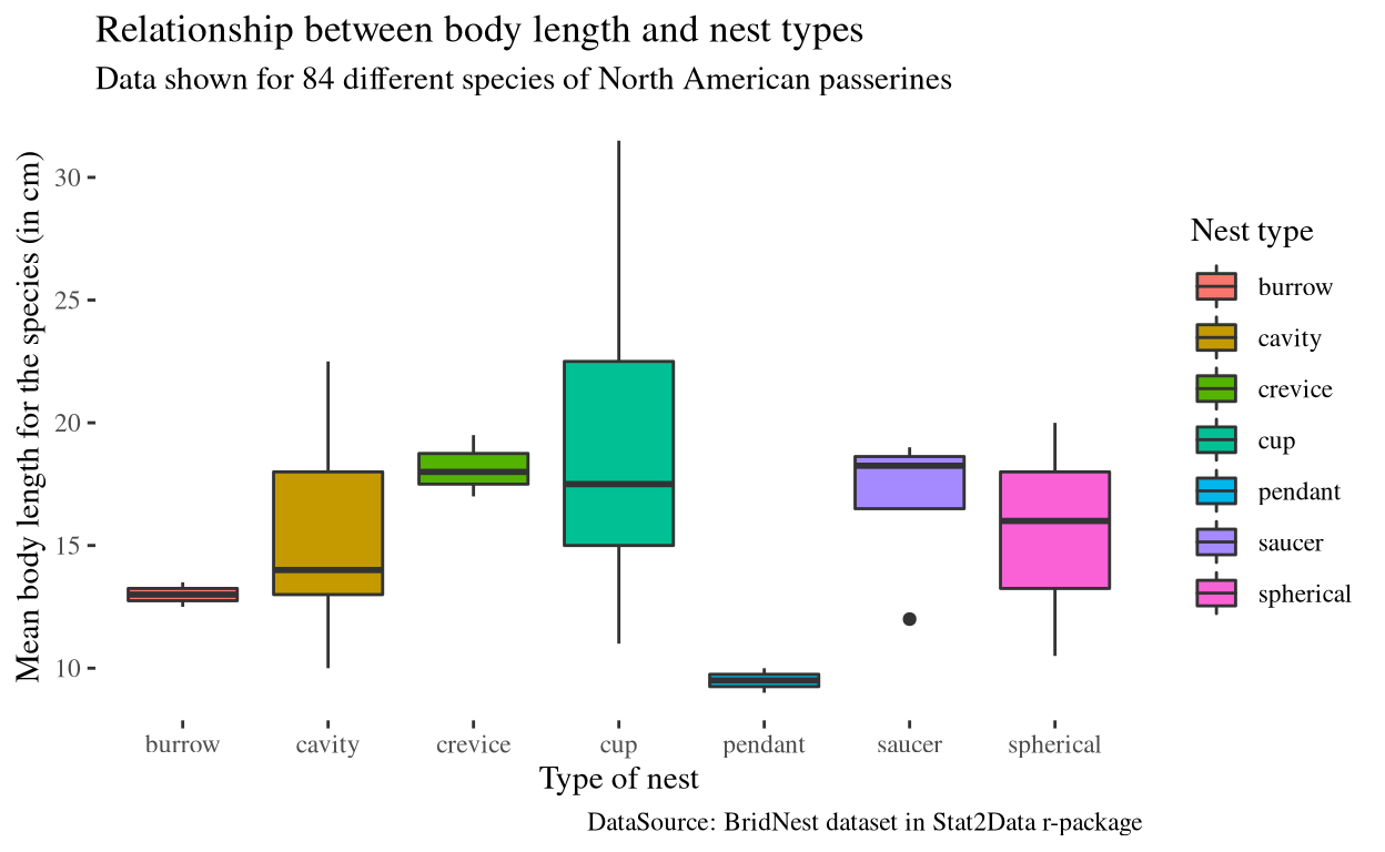
theme_wsj()
theme_wsj(): Theme based on the plots in The Wall Street Journal
Show code
ggplot(BirdNest, aes(Nesttype, Length, fill = Nesttype)) + geom_boxplot() +
  labs(x= "Type of nest", y= "Mean body length for the species (in cm)",
       fill= "Nest type", title= "Relationship between body length and nest types",
       subtitle = "Data shown for 84 different species of North American passerines",
       caption= "DataSource: BridNest dataset in Stat2Data r-package") +
  theme_wsj() + theme(text = element_text(size = 6)) #size is reduced to accommodate the graph in the tab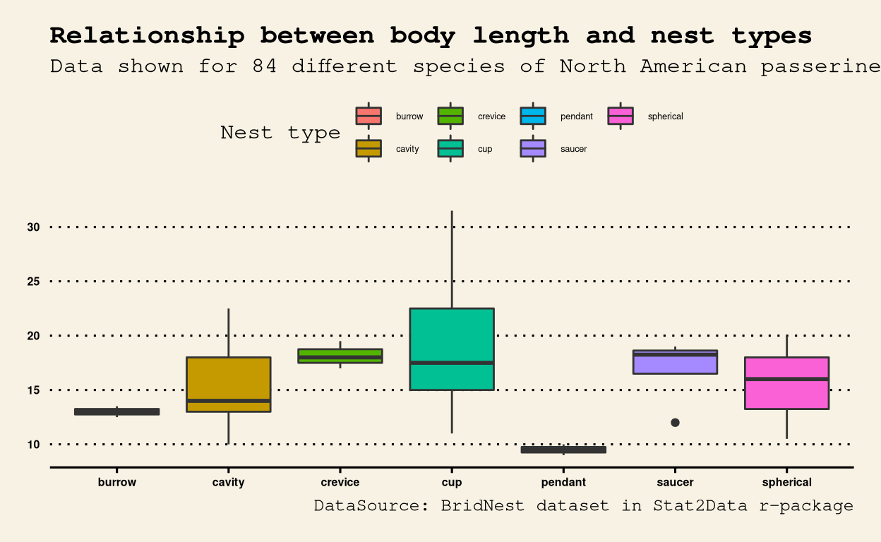
Changing colour palettes in ggplot2
Apart from ready to use themes, there are also ready to use colour palettes which we can use. A colour palette contains a set of pre-defined colours which will be applied to the different geometries present in a graph.
Choosing a good colour palette is important as it helps us to represent data in a better way and at the same time, it also makes the graph easier to read for people with colour blindness. Let us see a few popular colour palette packages used in R.
viridis package
viridis package is a popularly used colour palette in R. It is aesthetically pleasing and well designed to improve readability for colour blind people. The virids package was developed by Bob Rudis, Noam Ross and Simon Garnier. There are eight different colour scales present in this package. The name of the tab denotes the colour scale present in this package.
#load viridis colour package
library(viridis)
viridis
Show code
ggplot(BirdNest, aes(Nesttype, Length, fill = Nesttype)) + geom_boxplot() +
  labs(x= "Type of nest", y= "Mean body length for the species (in cm)",
       fill= "Nest type", title= "Relationship between body length and nest types",
       subtitle = "Data shown for 84 different species of North American passerines",
       caption= "DataSource: BridNest dataset in Stat2Data r-package") +
  theme_bw() + scale_fill_viridis(discrete = TRUE, option = "viridis")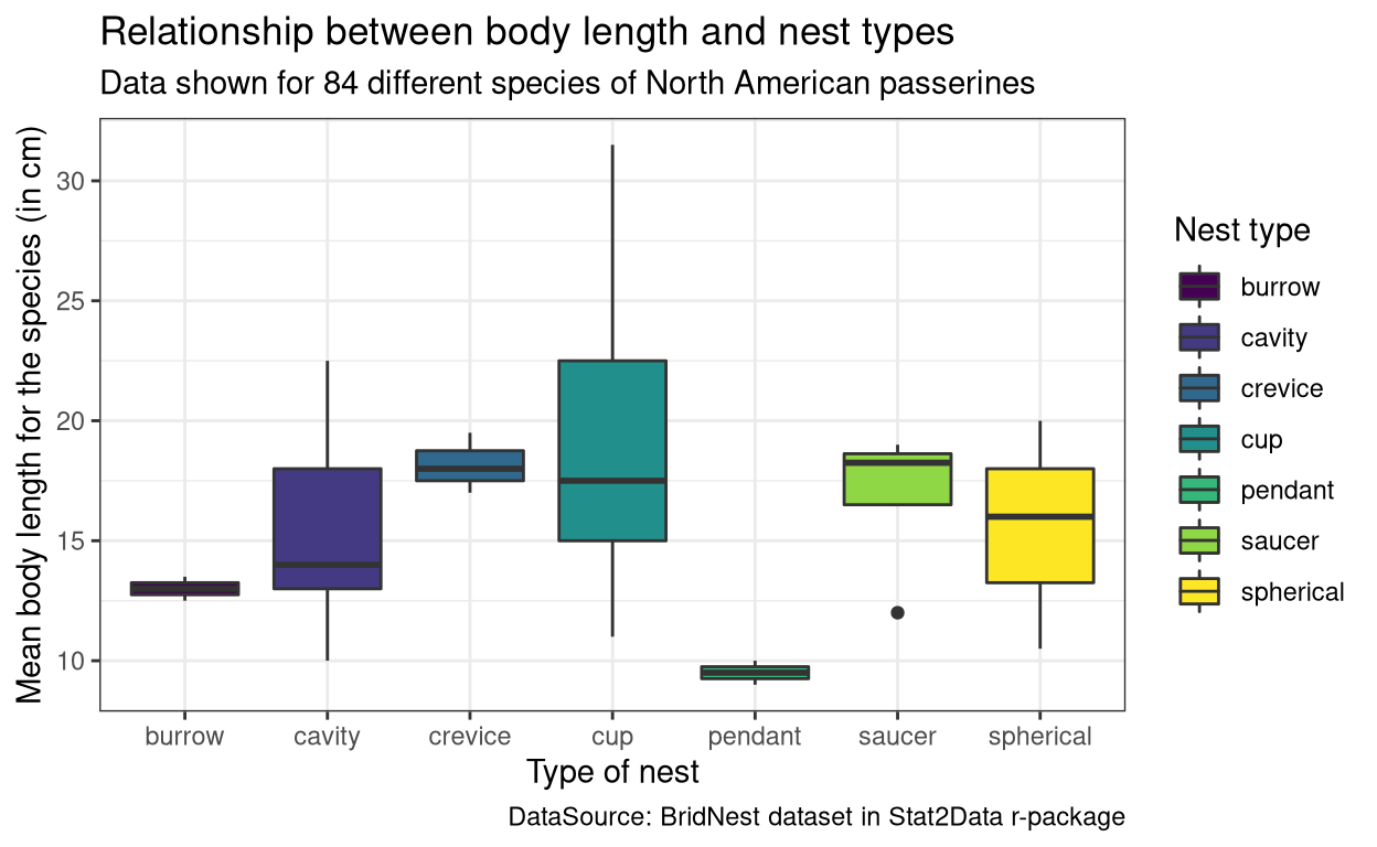
magma
Show code
ggplot(BirdNest, aes(Nesttype, Length, fill = Nesttype)) + geom_boxplot() +
  labs(x= "Type of nest", y= "Mean body length for the species (in cm)",
       fill= "Nest type", title= "Relationship between body length and nest types",
       subtitle = "Data shown for 84 different species of North American passerines",
       caption= "DataSource: BridNest dataset in Stat2Data r-package") +
  theme_bw() + scale_fill_viridis(discrete = TRUE, option = "magma")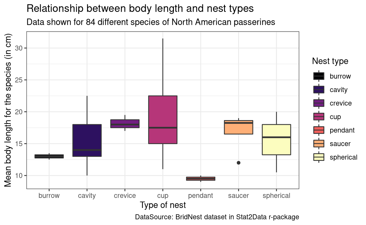
plasma
Show code
ggplot(BirdNest, aes(Nesttype, Length, fill = Nesttype)) + geom_boxplot() +
  labs(x= "Type of nest", y= "Mean body length for the species (in cm)",
       fill= "Nest type", title= "Relationship between body length and nest types",
       subtitle = "Data shown for 84 different species of North American passerines",
       caption= "DataSource: BridNest dataset in Stat2Data r-package") +
  theme_bw() + scale_fill_viridis(discrete = TRUE, option = "plasma")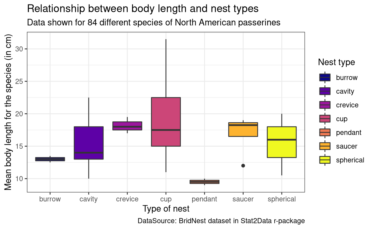
inferno
Show code
ggplot(BirdNest, aes(Nesttype, Length, fill = Nesttype)) + geom_boxplot() +
  labs(x= "Type of nest", y= "Mean body length for the species (in cm)",
       fill= "Nest type", title= "Relationship between body length and nest types",
       subtitle = "Data shown for 84 different species of North American passerines",
       caption= "DataSource: BridNest dataset in Stat2Data r-package") +
  theme_bw() + scale_fill_viridis(discrete = TRUE, option = "inferno")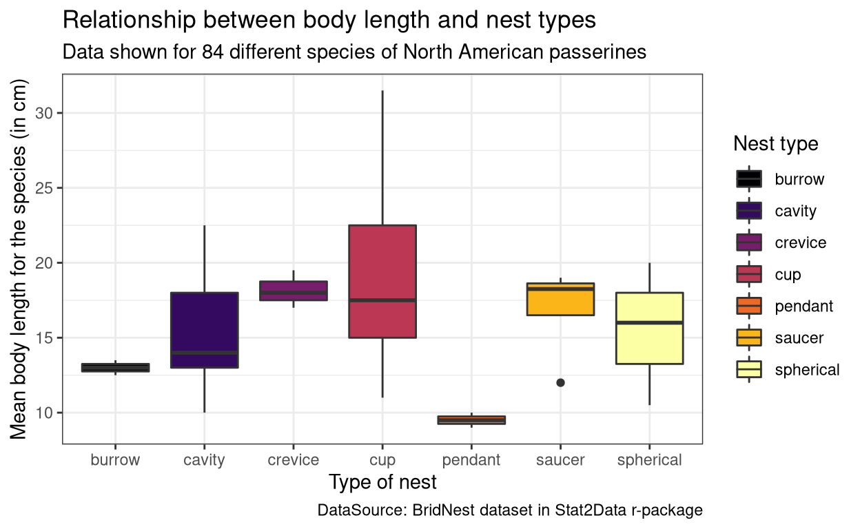
cividis
Show code
ggplot(BirdNest, aes(Nesttype, Length, fill = Nesttype)) + geom_boxplot() +
  labs(x= "Type of nest", y= "Mean body length for the species (in cm)",
       fill= "Nest type", title= "Relationship between body length and nest types",
       subtitle = "Data shown for 84 different species of North American passerines",
       caption= "DataSource: BridNest dataset in Stat2Data r-package") +
  theme_bw() + scale_fill_viridis(discrete = TRUE, option = "cividis")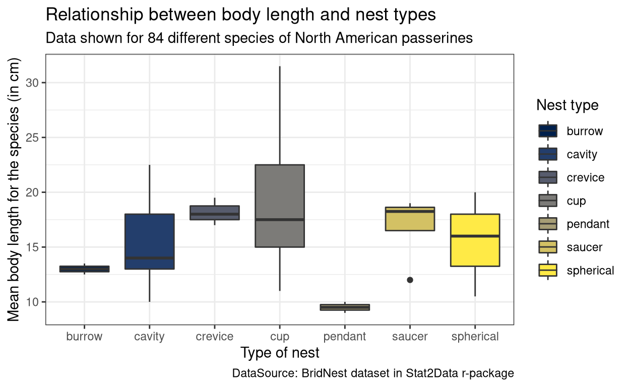
mako
Show code
ggplot(BirdNest, aes(Nesttype, Length, fill = Nesttype)) + geom_boxplot() +
  labs(x= "Type of nest", y= "Mean body length for the species (in cm)",
       fill= "Nest type", title= "Relationship between body length and nest types",
       subtitle = "Data shown for 84 different species of North American passerines",
       caption= "DataSource: BridNest dataset in Stat2Data r-package") +
  theme_bw() + scale_fill_viridis(discrete = TRUE, option = "mako")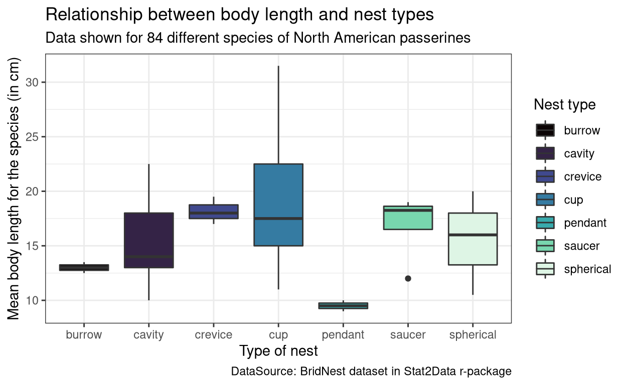
rocket
Show code
ggplot(BirdNest, aes(Nesttype, Length, fill = Nesttype)) + geom_boxplot() +
  labs(x= "Type of nest", y= "Mean body length for the species (in cm)",
       fill= "Nest type", title= "Relationship between body length and nest types",
       subtitle = "Data shown for 84 different species of North American passerines",
       caption= "DataSource: BridNest dataset in Stat2Data r-package") +
  theme_bw() + scale_fill_viridis(discrete = TRUE, option = "rocket")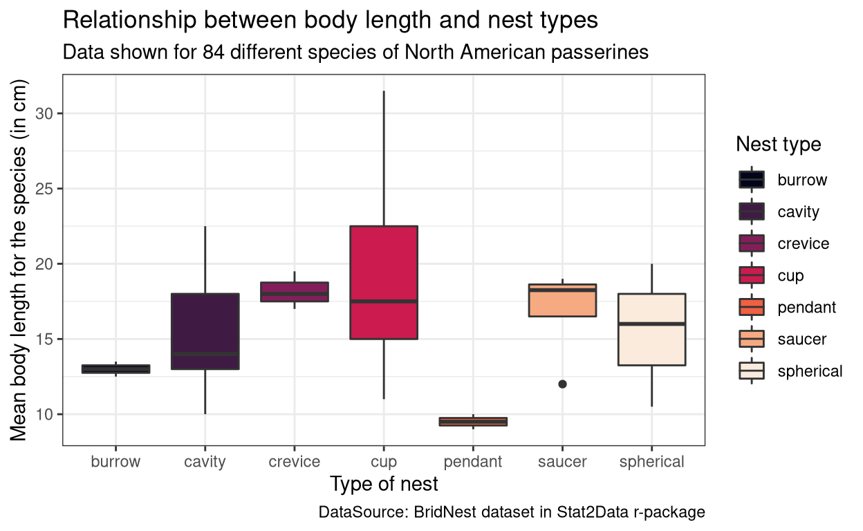
turbo
Show code
ggplot(BirdNest, aes(Nesttype, Length, fill = Nesttype)) + geom_boxplot() +
  labs(x= "Type of nest", y= "Mean body length for the species (in cm)",
       fill= "Nest type", title= "Relationship between body length and nest types",
       subtitle = "Data shown for 84 different species of North American passerines",
       caption= "DataSource: BridNest dataset in Stat2Data r-package") +
  theme_bw() + scale_fill_viridis(discrete = TRUE, option = "turbo")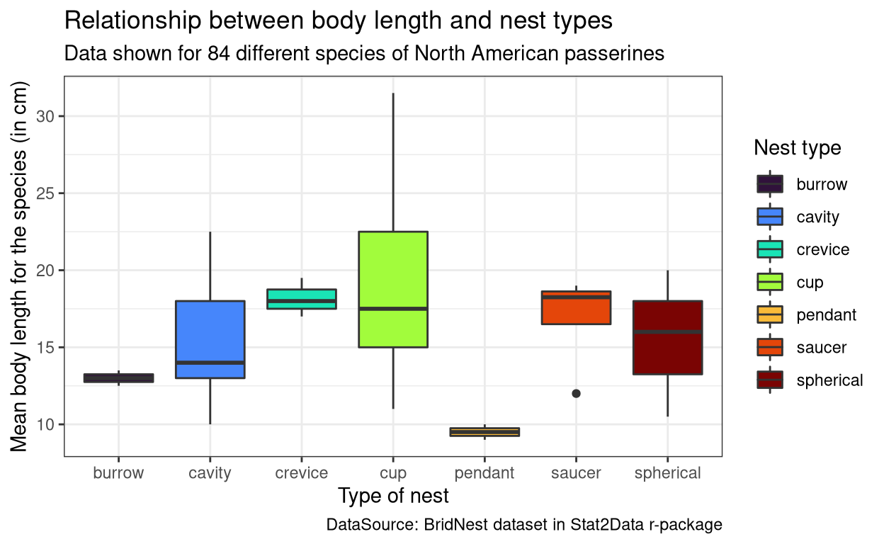
wesanderson package
If you like your colours distinctive and narrative, just like how American film-maker Mr. Wes Anderson would like it, then try the wesanderson package. Relive the The Grand Budapest Hotel moments through your graphs. The wesandreson package was developed by Karthik Ram. There are a total of 19 colour palettes present in this package. We will see a subset of them. All colour scales in this package are available here. The name of the tab denotes the colour scale used. The data used in this plot is the penguin dataset present in the package palmerpenguins.
#install and load wesanderson and palmerpenguins package
install.packages("wesanderson")
install.packages("palmerpenguins")
library(wesanderson)
library(palmerpenguins)
data("penguins") #load the penguins dataset
GrandBudapest1
Show code
ggplot(data = penguins, aes(x = species, y = body_mass_g, fill = species)) +
  labs(x= "Species", y= "Body mass (g)",
       fill= "Nest type", title= "Body mass in three diferent species of penguins",
       subtitle = "Penguins observed on islands near Palmer Station, Antarctica",
       caption= "DataSource: penguins dataset in palmerpenguins r-package") + geom_boxplot() +
  theme_bw() + scale_fill_manual(values = wes_palette("GrandBudapest1", n = 3))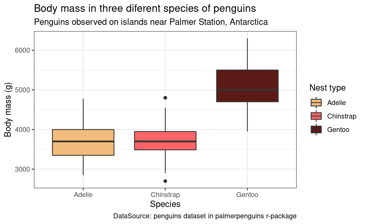
BottleRocket2
Show code
ggplot(data = penguins, aes(x = species, y = body_mass_g, fill = species)) +
  labs(x= "Species", y= "Body mass (g)",
       fill= "Nest type", title= "Body mass in three diferent species of penguins",
       subtitle = "Penguins observed on islands near Palmer Station, Antarctica",
       caption= "DataSource: penguins dataset in palmerpenguins r-package") + geom_boxplot() +
  theme_bw() + scale_fill_manual(values = wes_palette("BottleRocket2", n = 3))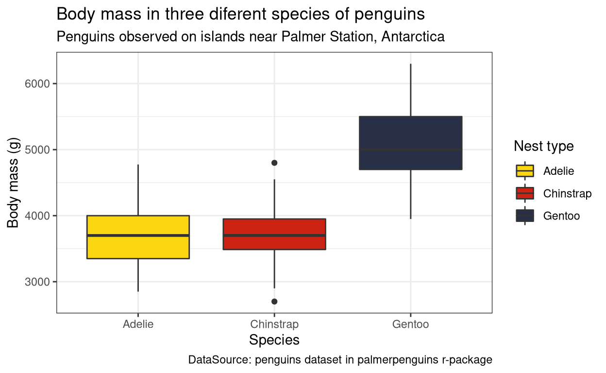
Rushmore1
Show code
ggplot(data = penguins, aes(x = species, y = body_mass_g, fill = species)) +
  labs(x= "Species", y= "Body mass (g)",
       fill= "Nest type", title= "Body mass in three diferent species of penguins",
       subtitle = "Penguins observed on islands near Palmer Station, Antarctica",
       caption= "DataSource: penguins dataset in palmerpenguins r-package") + geom_boxplot() +
  theme_bw() + scale_fill_manual(values = wes_palette("Rushmore1", n = 3))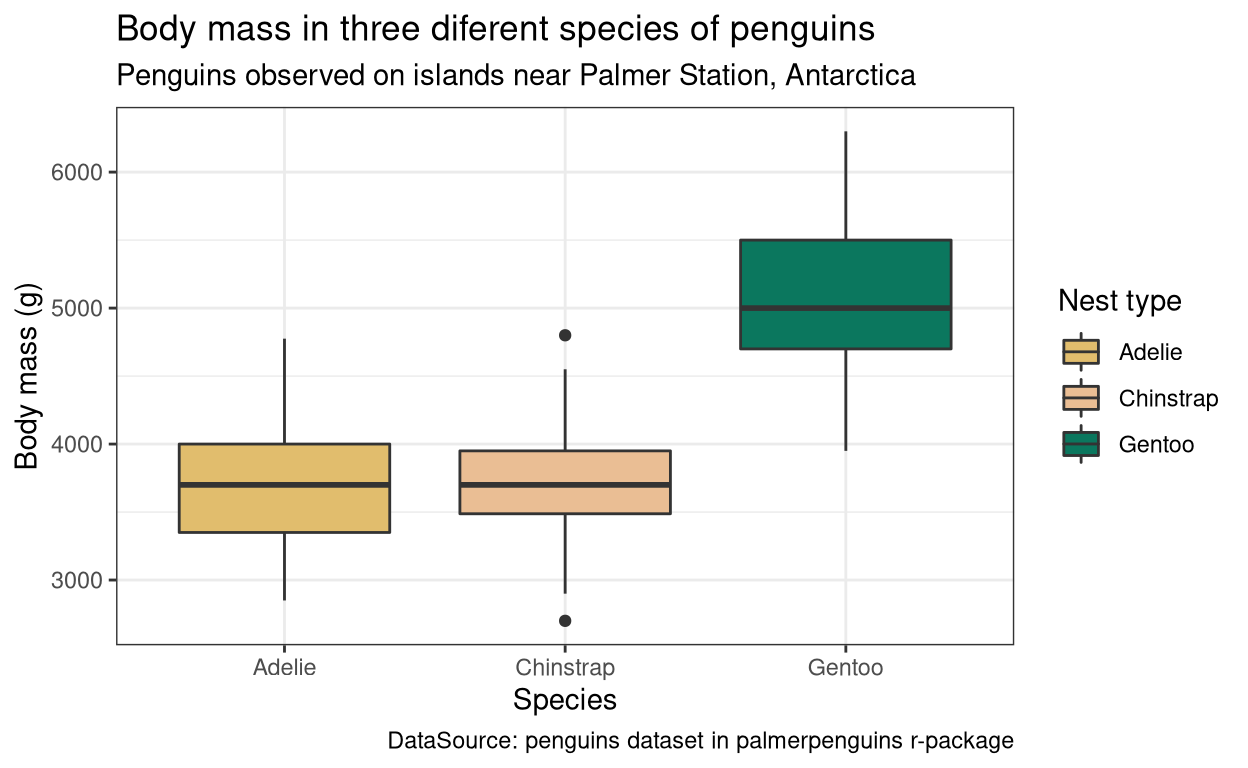
Royal1
Show code
ggplot(data = penguins, aes(x = species, y = body_mass_g, fill = species)) +
  labs(x= "Species", y= "Body mass (g)",
       fill= "Nest type", title= "Body mass in three diferent species of penguins",
       subtitle = "Penguins observed on islands near Palmer Station, Antarctica",
       caption= "DataSource: penguins dataset in palmerpenguins r-package") + geom_boxplot() +
  theme_bw() + scale_fill_manual(values = wes_palette("Royal1", n = 3))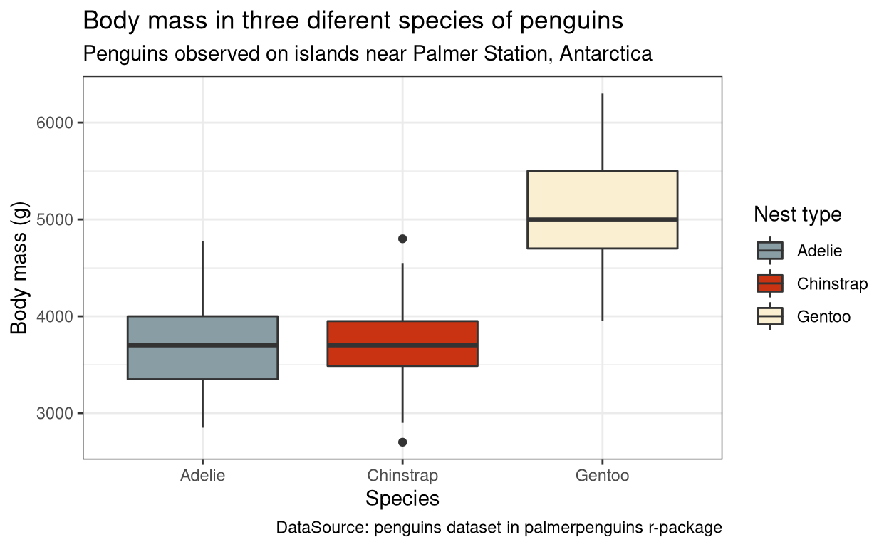
Zissou1
Show code
ggplot(data = penguins, aes(x = species, y = body_mass_g, fill = species)) +
  labs(x= "Species", y= "Body mass (g)",
       fill= "Nest type", title= "Body mass in three diferent species of penguins",
       subtitle = "Penguins observed on islands near Palmer Station, Antarctica",
       caption= "DataSource: penguins dataset in palmerpenguins r-package") + geom_boxplot() +
  theme_bw() + scale_fill_manual(values = wes_palette("Zissou1", n = 3))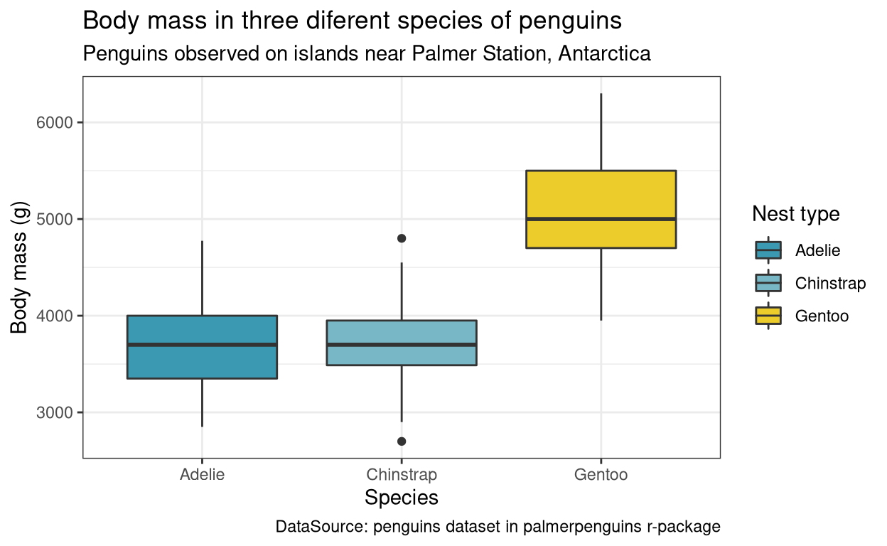
Darjeeling2
Show code
ggplot(data = penguins, aes(x = species, y = body_mass_g, fill = species)) +
  labs(x= "Species", y= "Body mass (g)",
       fill= "Nest type", title= "Body mass in three diferent species of penguins",
       subtitle = "Penguins observed on islands near Palmer Station, Antarctica",
       caption= "DataSource: penguins dataset in palmerpenguins r-package") + geom_boxplot() +
  theme_bw() + scale_fill_manual(values = wes_palette("Darjeeling2", n = 3))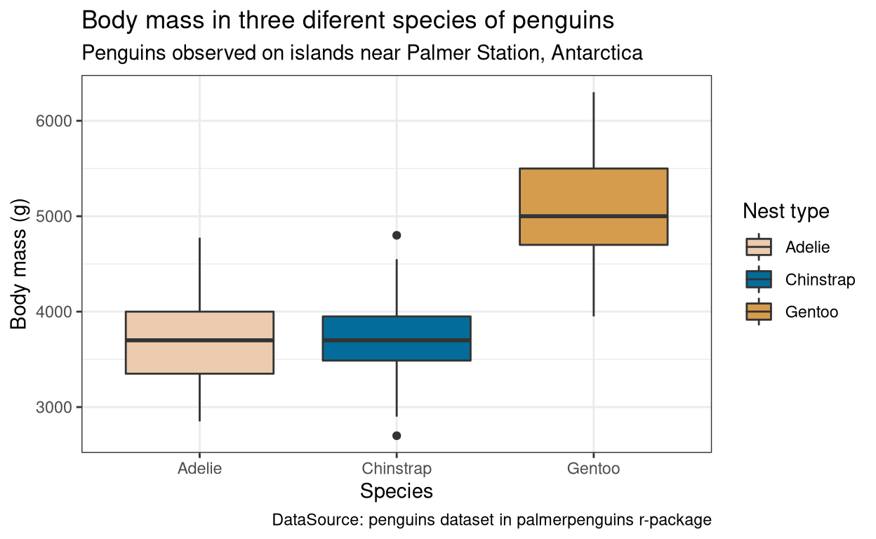
IsleofDogs1
Show code
ggplot(data = penguins, aes(x = species, y = body_mass_g, fill = species)) +
  labs(x= "Species", y= "Body mass (g)",
       fill= "Nest type", title= "Body mass in three diferent species of penguins",
       subtitle = "Penguins observed on islands near Palmer Station, Antarctica",
       caption= "DataSource: penguins dataset in palmerpenguins r-package") + geom_boxplot() +
  theme_bw() + scale_fill_manual(values = wes_palette("IsleofDogs1", n = 3))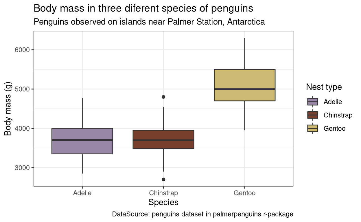
ggsci package
If you want high-quality colour palettes reflecting scientific journal styles then you can try the ggsci package. The ggsci package was developed by Dr. Nan Xiao and Dr. Miaozhu Li. All colour scales in this package are available in package webpage. The descriptions of the colour scales were also taken from the package webpage. The name of the tab denotes the colour scale used.
#load ggsci package
library(ggsci)
scale_fill_npg()
The NPG palette is inspired by the plots in the journals published by Nature Publishing Group.
Show code
ggplot(BirdNest, aes(Nesttype, Length, fill = Nesttype)) + geom_boxplot() +
  labs(x= "Type of nest", y= "Mean body length for the species (in cm)",
       fill= "Nest type", title= "Relationship between body length and nest types",
       subtitle = "Data shown for 84 different species of North American passerines",
       caption= "DataSource: BridNest dataset in Stat2Data r-package") +
  theme_bw() + scale_fill_npg()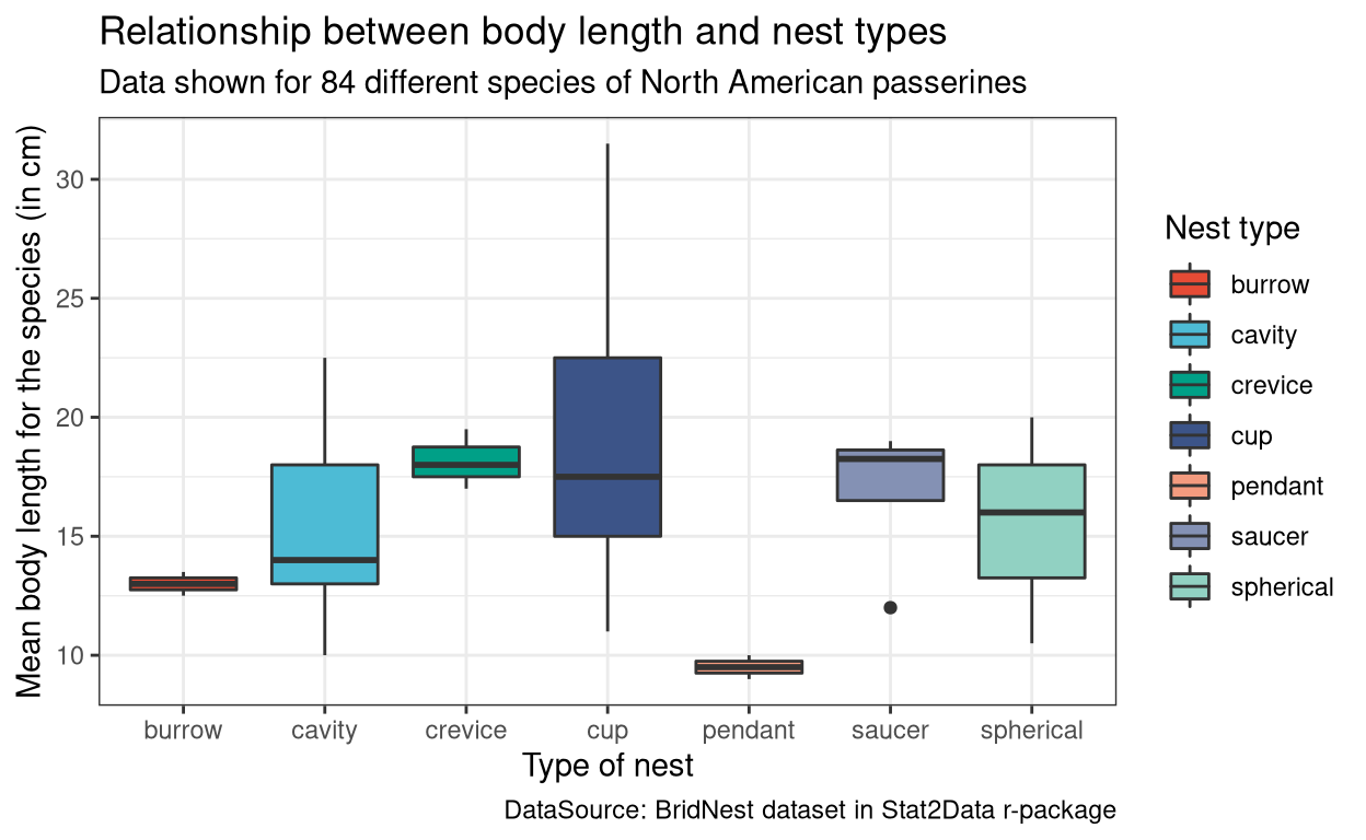
scale_fill_aaas()
The AAAS palette is inspired by the plots in the journals published by American Association for the Advancement of Science.
Show code
ggplot(BirdNest, aes(Nesttype, Length, fill = Nesttype)) + geom_boxplot() +
  labs(x= "Type of nest", y= "Mean body length for the species (in cm)",
       fill= "Nest type", title= "Relationship between body length and nest types",
       subtitle = "Data shown for 84 different species of North American passerines",
       caption= "DataSource: BridNest dataset in Stat2Data r-package") +
  theme_bw() + scale_fill_aaas()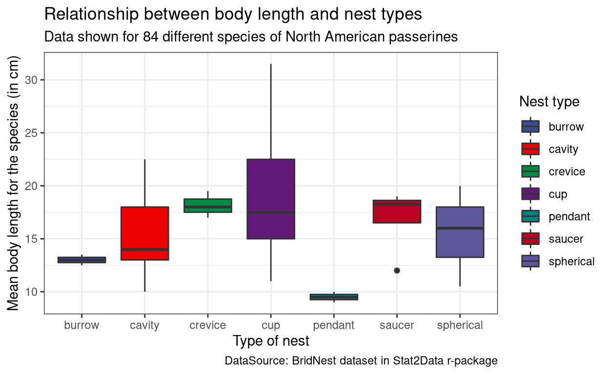
scale_fill_nejm()
The NEJM palette is inspired by the plots in The New England Journal of Medicine.
Show code
ggplot(BirdNest, aes(Nesttype, Length, fill = Nesttype)) + geom_boxplot() +
  labs(x= "Type of nest", y= "Mean body length for the species (in cm)",
       fill= "Nest type", title= "Relationship between body length and nest types",
       subtitle = "Data shown for 84 different species of North American passerines",
       caption= "DataSource: BridNest dataset in Stat2Data r-package") +
  theme_bw() + scale_fill_nejm()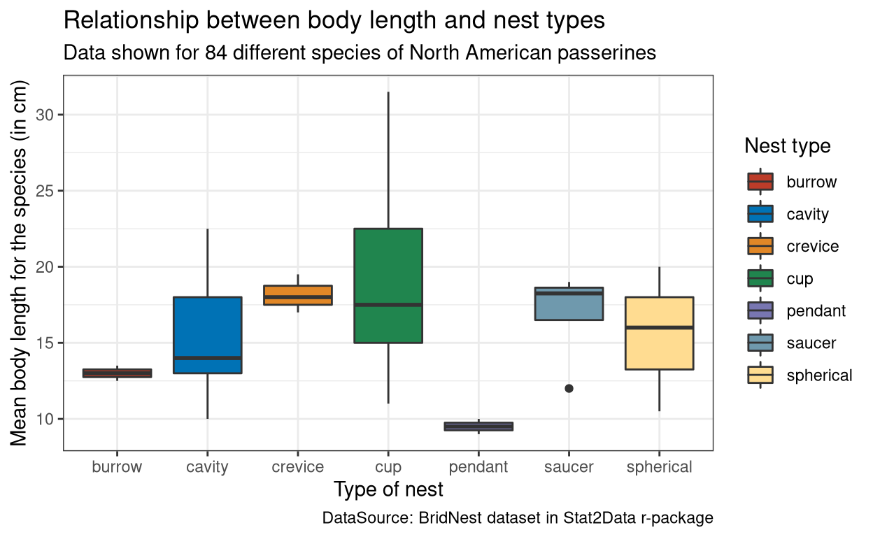
scale_fill_lancet()
The Lancet palette is inspired by the plots in Lancet journals, such as Lancet Oncology.
Show code
ggplot(BirdNest, aes(Nesttype, Length, fill = Nesttype)) + geom_boxplot() +
  labs(x= "Type of nest", y= "Mean body length for the species (in cm)",
       fill= "Nest type", title= "Relationship between body length and nest types",
       subtitle = "Data shown for 84 different species of North American passerines",
       caption= "DataSource: BridNest dataset in Stat2Data r-package") +
  theme_bw() + scale_fill_lancet()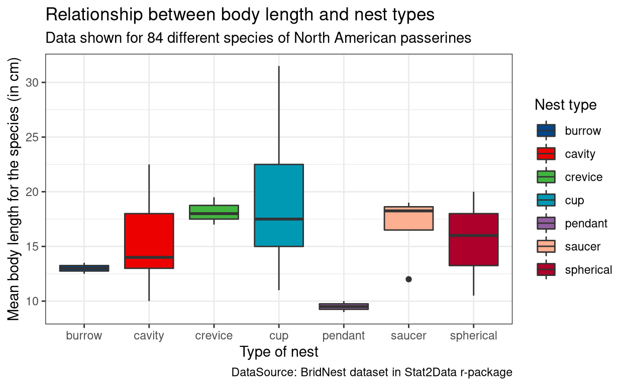
scale_fill_jama()
The JAMA palette is inspired by the plots in The Journal of the American Medical Association.
Show code
ggplot(BirdNest, aes(Nesttype, Length, fill = Nesttype)) + geom_boxplot() +
  labs(x= "Type of nest", y= "Mean body length for the species (in cm)",
       fill= "Nest type", title= "Relationship between body length and nest types",
       subtitle = "Data shown for 84 different species of North American passerines",
       caption= "DataSource: BridNest dataset in Stat2Data r-package") +
  theme_bw() + scale_fill_jama()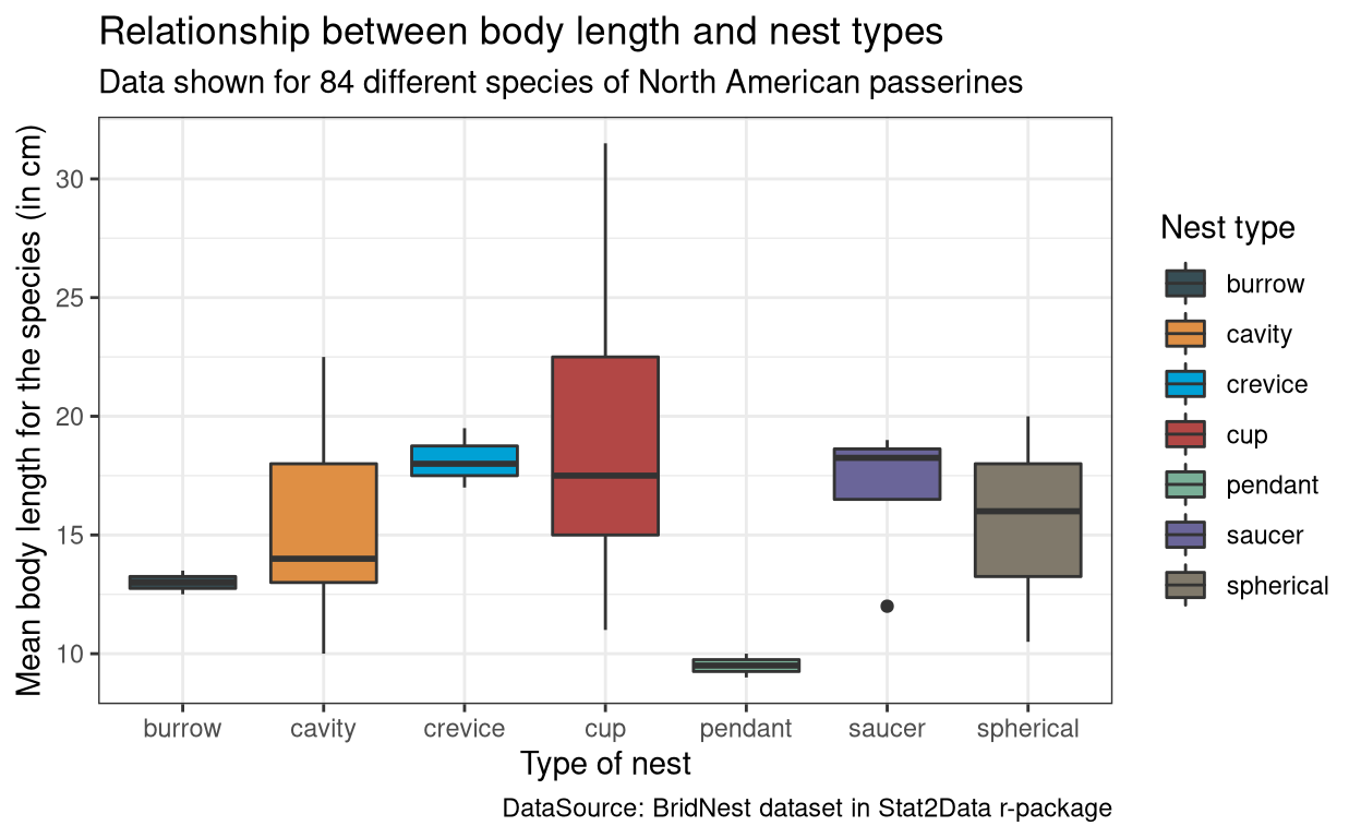
scale_fill_jco()
The JCO palette is inspired by the the plots in Journal of Clinical Oncology.
Show code
ggplot(BirdNest, aes(Nesttype, Length, fill = Nesttype)) + geom_boxplot() +
  labs(x= "Type of nest", y= "Mean body length for the species (in cm)",
       fill= "Nest type", title= "Relationship between body length and nest types",
       subtitle = "Data shown for 84 different species of North American passerines",
       caption= "DataSource: BridNest dataset in Stat2Data r-package") +
  theme_bw() + scale_fill_jco()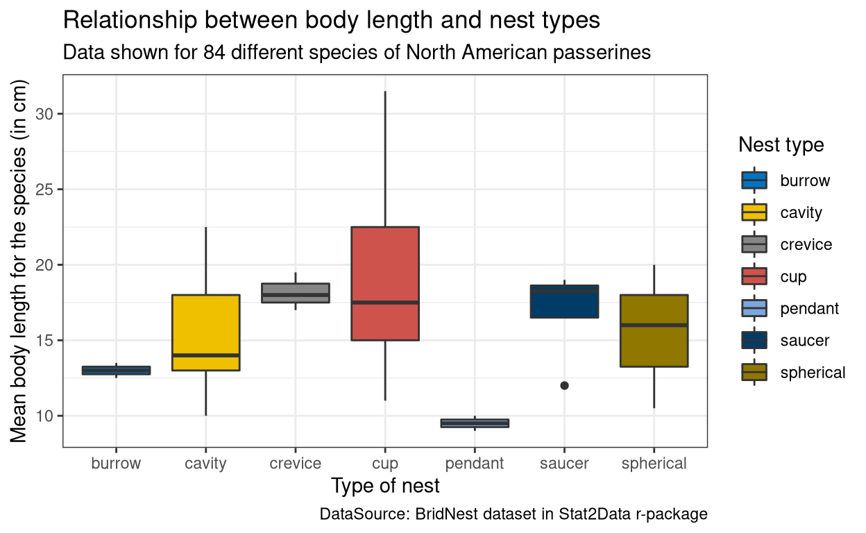
scale_fill_ucscgb()
The UCSCGB palette is from the colors used by UCSC Genome Browser for representing chromosomes. This palette has been intensively used in visualizations produced by Circos.
Show code
ggplot(BirdNest, aes(Nesttype, Length, fill = Nesttype)) + geom_boxplot() +
  labs(x= "Type of nest", y= "Mean body length for the species (in cm)",
       fill= "Nest type", title= "Relationship between body length and nest types",
       subtitle = "Data shown for 84 different species of North American passerines",
       caption= "DataSource: BridNest dataset in Stat2Data r-package") +
  theme_bw() + scale_fill_ucscgb()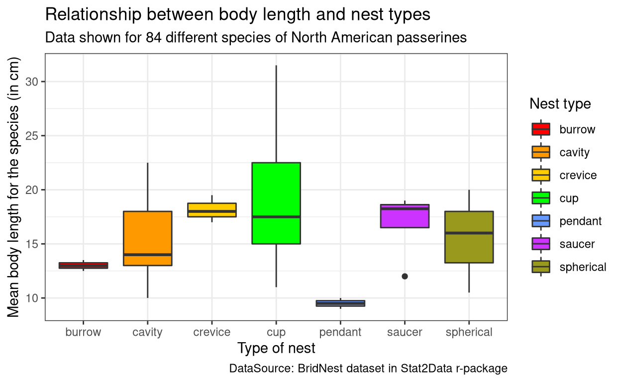
scale_fill_d3()
The D3 palette is from the categorical colors used by D3.js (version 3.x and before). There are four palette types
(category10, category20, category20b, category20c)available.
Show code
ggplot(BirdNest, aes(Nesttype, Length, fill = Nesttype)) + geom_boxplot() +
  labs(x= "Type of nest", y= "Mean body length for the species (in cm)",
       fill= "Nest type", title= "Relationship between body length and nest types",
       subtitle = "Data shown for 84 different species of North American passerines",
       caption= "DataSource: BridNest dataset in Stat2Data r-package") +
  theme_bw() + scale_fill_d3(palette = "category10")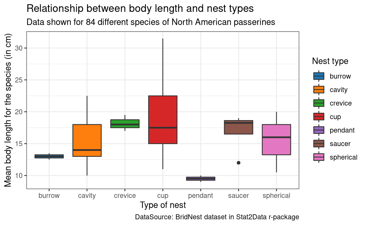
scale_fill_locuszoom()
The LocusZoom palette is based on the colors used by LocusZoom.
Show code
ggplot(BirdNest, aes(Nesttype, Length, fill = Nesttype)) + geom_boxplot() +
  labs(x= "Type of nest", y= "Mean body length for the species (in cm)",
       fill= "Nest type", title= "Relationship between body length and nest types",
       subtitle = "Data shown for 84 different species of North American passerines",
       caption= "DataSource: BridNest dataset in Stat2Data r-package") +
  theme_bw() + scale_fill_locuszoom()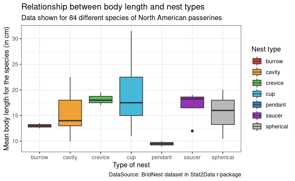
scale_fill_igv()
The IGV palette is from the colors used by Integrative Genomics Viewer for representing chromosomes. There are two palette types (default, alternating) available.
Show code
ggplot(BirdNest, aes(Nesttype, Length, fill = Nesttype)) + geom_boxplot() +
  labs(x= "Type of nest", y= "Mean body length for the species (in cm)",
       fill= "Nest type", title= "Relationship between body length and nest types",
       subtitle = "Data shown for 84 different species of North American passerines",
       caption= "DataSource: BridNest dataset in Stat2Data r-package") +
  theme_bw() + scale_fill_igv()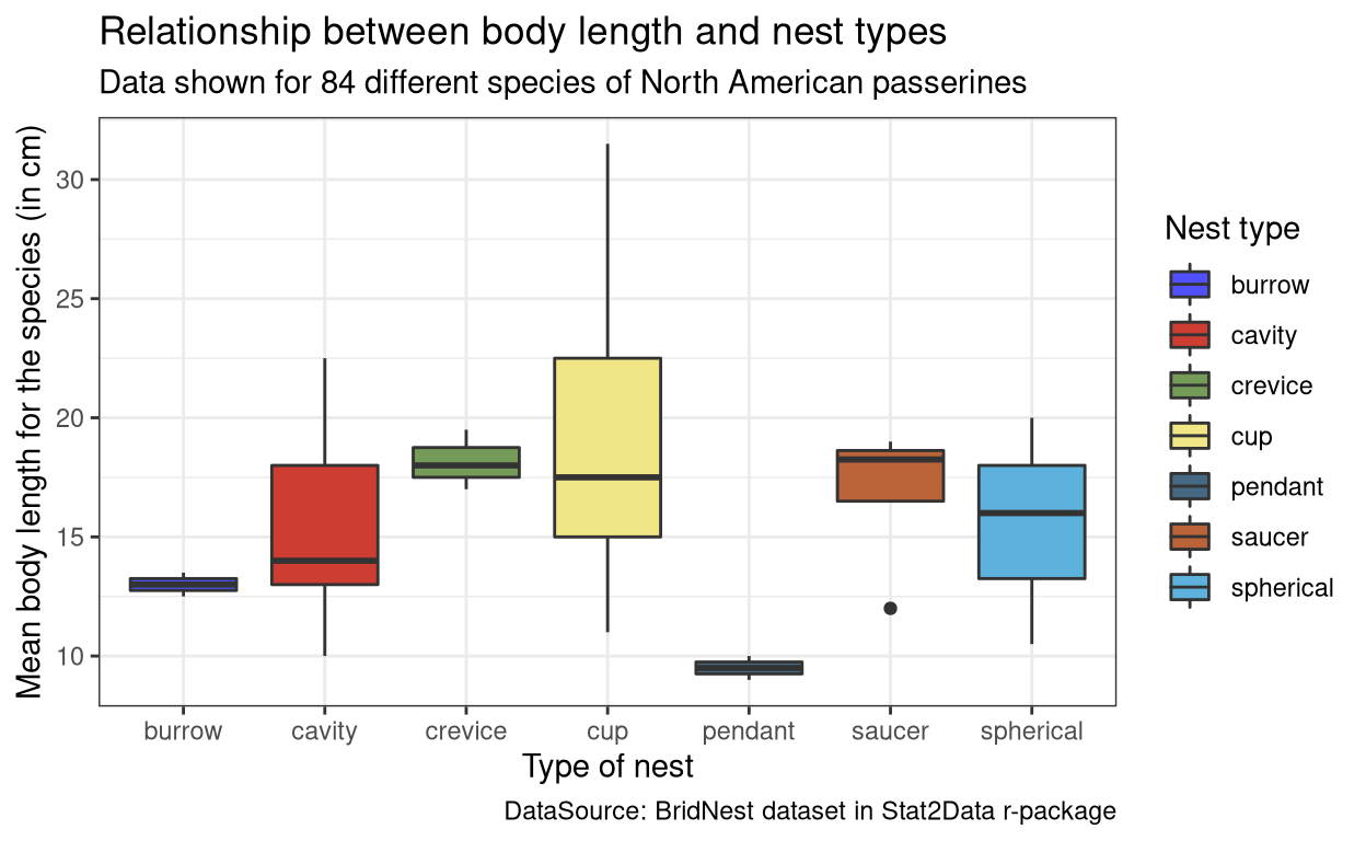
scale_fill_uchicago()
The UChicago palette is based on the colors used by the University of Chicago. There are three palette types (default, light, dark) available.
Show code
ggplot(BirdNest, aes(Nesttype, Length, fill = Nesttype)) + geom_boxplot() +
  labs(x= "Type of nest", y= "Mean body length for the species (in cm)",
       fill= "Nest type", title= "Relationship between body length and nest types",
       subtitle = "Data shown for 84 different species of North American passerines",
       caption= "DataSource: BridNest dataset in Stat2Data r-package") +
  theme_bw() + scale_fill_uchicago()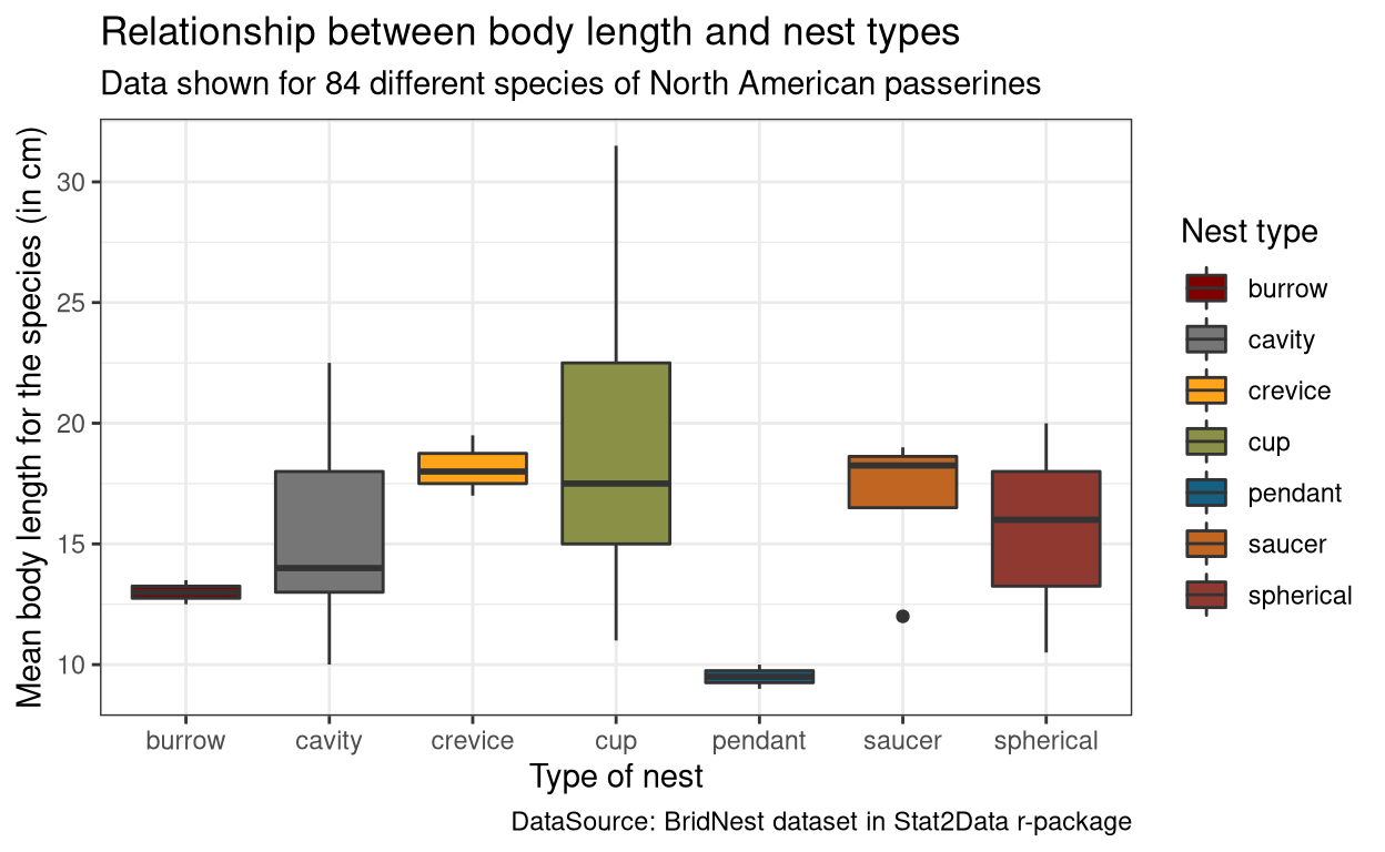
scale_fill_startrek()
This palette is inspired by the (uniform) colors in Star Trek.
Show code
ggplot(BirdNest, aes(Nesttype, Length, fill = Nesttype)) + geom_boxplot() +
  labs(x= "Type of nest", y= "Mean body length for the species (in cm)",
       fill= "Nest type", title= "Relationship between body length and nest types",
       subtitle = "Data shown for 84 different species of North American passerines",
       caption= "DataSource: BridNest dataset in Stat2Data r-package") +
  theme_bw() + scale_fill_startrek()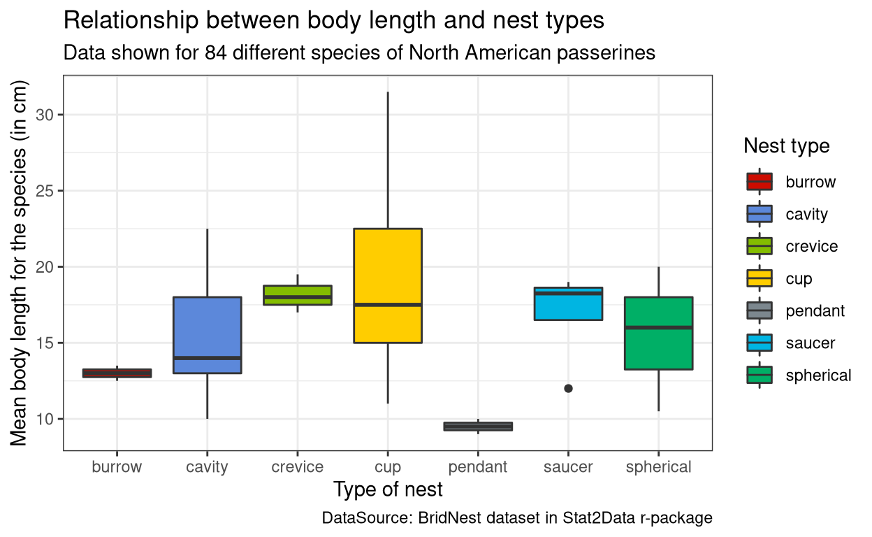
scale_fill_tron()
This palette is inspired by the colors used in Tron Legacy. It is suitable for displaying data when using a dark theme.
Show code
ggplot(BirdNest, aes(Nesttype, Length, fill = Nesttype)) + geom_boxplot() +
  labs(x= "Type of nest", y= "Mean body length for the species (in cm)",
       fill= "Nest type", title= "Relationship between body length and nest types",
       subtitle = "Data shown for 84 different species of North American passerines",
       caption= "DataSource: BridNest dataset in Stat2Data r-package") +
  theme_bw() + scale_fill_tron()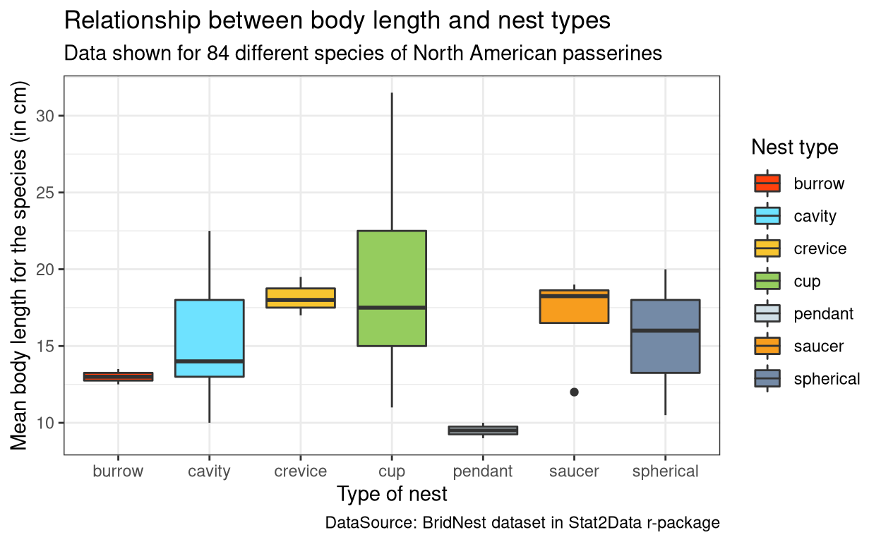
scale_fill_futurama()
This palette is inspired by the colors used in the TV show Futurama.
Show code
ggplot(BirdNest, aes(Nesttype, Length, fill = Nesttype)) + geom_boxplot() +
  labs(x= "Type of nest", y= "Mean body length for the species (in cm)",
       fill= "Nest type", title= "Relationship between body length and nest types",
       subtitle = "Data shown for 84 different species of North American passerines",
       caption= "DataSource: BridNest dataset in Stat2Data r-package") +
  theme_bw() + scale_fill_futurama()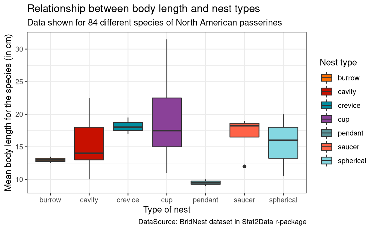
scale_fill_rickandmorty()
This palette is inspired by the colors used in the TV show Rick and Morty.
Show code
ggplot(BirdNest, aes(Nesttype, Length, fill = Nesttype)) + geom_boxplot() +
  labs(x= "Type of nest", y= "Mean body length for the species (in cm)",
       fill= "Nest type", title= "Relationship between body length and nest types",
       subtitle = "Data shown for 84 different species of North American passerines",
       caption= "DataSource: BridNest dataset in Stat2Data r-package") +
  theme_bw() + scale_fill_rickandmorty()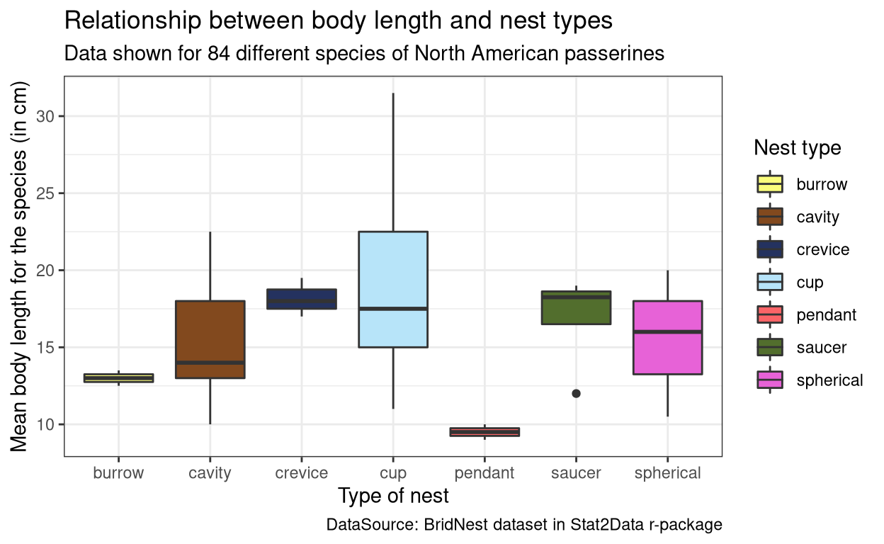
scale_fill_simpsons()
This palette is inspired by the colors used in the TV show The Simpsons.
Show code
ggplot(BirdNest, aes(Nesttype, Length, fill = Nesttype)) + geom_boxplot() +
  labs(x= "Type of nest", y= "Mean body length for the species (in cm)",
       fill= "Nest type", title= "Relationship between body length and nest types",
       subtitle = "Data shown for 84 different species of North American passerines",
       caption= "DataSource: BridNest dataset in Stat2Data r-package") +
  theme_bw() + scale_fill_simpsons()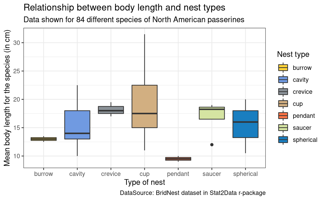
Customizing the theme()
A ggplot theme is made up of different elements and it’s functions. For e.g. plot.title() element allows you to modify the title of the graph using the element function element_text(). In this way, we can change the font size, font family, text colour etc. of the title of the plot. So let us begin customising our graph. We will be reusing the BirdNest dataset for the graphs.
1. Customizing text elements using element_text()
All text elements can be customized using the element function element_text(). The syntax for element_text() is as follows
element_text(
  family = NULL, #insert family font name, e.g. "Times"
  face = NULL,  #font face ("plain", "italic", "bold", "bold.italic")
  colour = NULL, #either from colours() or hex code inside ""
  size = NULL, #text size (in pts)
  hjust = NULL, #horizontal justification values 0 or 1
  vjust = NULL, #vertical justification values 0 or 1
  angle = NULL, #angle in degrees
  lineheight = NULL, #distance between text and axis line
  color = NULL, #same function as colour
  margin = NULL,
  debug = NULL,
  inherit.blank = FALSE
)
Before
Show code
p <- ggplot(BirdNest, aes(No.eggs, Totcare, colour = Nesttype)) + geom_point() +
    labs(x= "Number of eggs", y= "Total care time (days)",
       title= "Relationship between number of eggs and total care time",
       subtitle = "Data shown for 84 different species of North American passerines",
       caption= "DataSource: BridNest dataset in Stat2Data r-package",
       colour = "Nest type")
p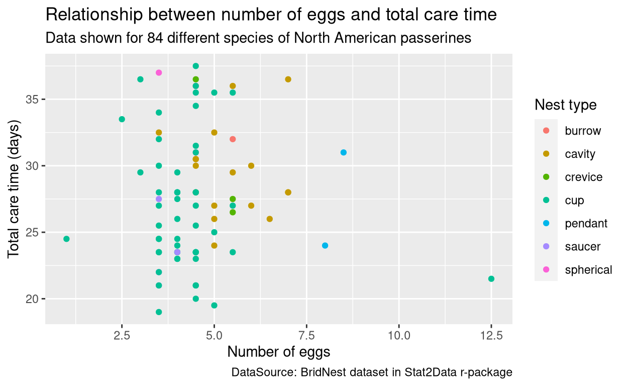
After
Show code
p <- ggplot(BirdNest, aes(No.eggs, Totcare, colour = Nesttype)) + geom_point() +
    labs(x= "Number of eggs", y= "Total care time (days)",
       title= "Relationship between number of eggs and total care time",
       subtitle = "Data shown for 84 different species of North American passerines",
       caption= "DataSource: BridNest dataset in Stat2Data r-package",
       colour = "Nest type")

#customizing text elements
p + theme(plot.title=element_text(size = 15,family = "Comic Sans MS",colour = "darkred",face = "bold"),
          plot.subtitle=element_text(size = 10,family = "Courier",colour= "blue",face= "italic"),
          plot.caption = element_text(size = 8,family = "Times",colour= "green",face="bold.italic", hjust=0),
          axis.text.x= element_text(size = 6,colour = "magenta", angle=20),
          axis.text.y= element_text(size = 6,colour = "darkblue", angle=30),
          axis.title.x = element_text(colour = "orchid"),
          axis.title.y = element_text(colour = "sienna"),
          legend.text = element_text(size = 8,colour = "darkgreen"),
          legend.title = element_text(size = 10,colour = "lightblue",face = "bold"))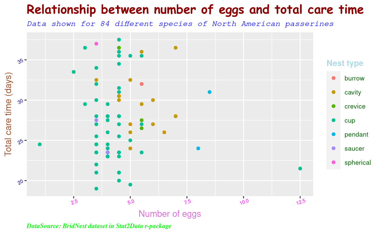
2. Customizing line elements using element_line()
Line elements include axes, grid lines, borders of the graph etc. All line elements can be customized using the element function element_line(). The syntax for element_line() is as follows
element_line(
  colour = NULL, #either from colours() or hex code inside ""
  size = NULL, #line size in mm units
  linetype = NULL, # eg: dashed, dotted etc
  lineend = NULL, #line end style (round, butt, square)
  color = NULL, #same function as colour
  arrow = NULL, #arrow specification
  inherit.blank = FALSE
)
Before
Show code
p <- ggplot(BirdNest, aes(Nesttype, Length, fill = Nesttype)) + geom_boxplot() +
  labs(x= "Type of nest", y= "Mean body length for the species (in cm)",
       fill= "Nest type", title= "Relationship between body length and nest types",
       subtitle = "Data shown for 84 different species of North American passerines",
       caption= "DataSource: BridNest dataset in Stat2Data r-package")
p
After
Show code
p <- ggplot(BirdNest, aes(Nesttype, Length, fill = Nesttype)) + geom_boxplot() +
  labs(x= "Type of nest", y= "Mean body length for the species (in cm)",
       fill= "Nest type", title= "Relationship between body length and nest types",
       subtitle = "Data shown for 84 different species of North American passerines",
       caption= "DataSource: BridNest dataset in Stat2Data r-package")

#customizing line elements
p + theme(panel.grid.major = element_line(colour = "red", size = 0.8, linetype = "dashed"),
          panel.grid.minor = element_line(colour = "blue",linetype = "twodash"),
          axis.line.x = element_line(colour = "darkred", arrow = arrow()),
          axis.line.y = element_line(colour = "darkblue"),
          axis.ticks = element_line(size = 5, colour = "yellow"),
          axis.ticks.length.y=unit(0.5, "cm")) #ticks positioned 0.5cm away from y axis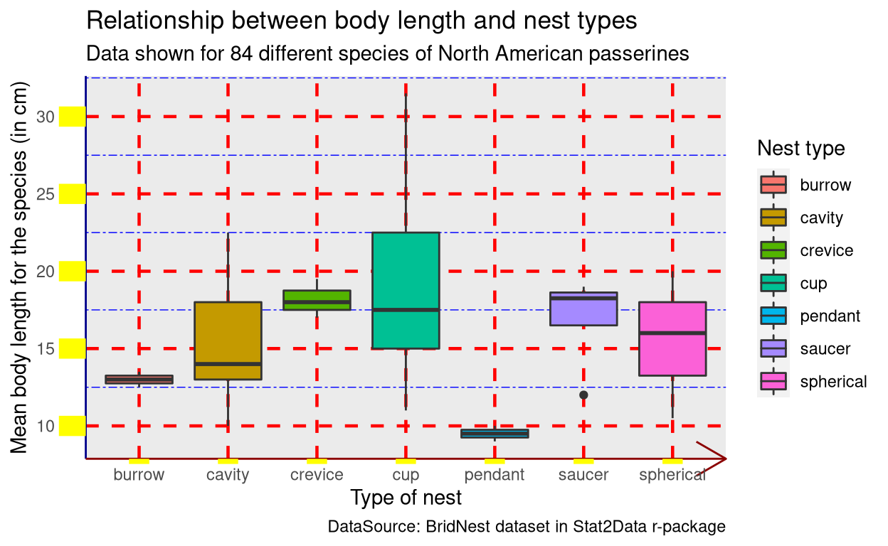
3. Customizing background elements using element_rect()
Background elements include plot, panel and legend backgrounds and their margins. All background elements can be customized using the element function element_rect(). The syntax for element_rect() is as follows
element_rect(
  fill = NULL, #fills colour
  colour = NULL, #colours the border
  size = NULL, #changes border size in mm units
  linetype = NULL, #changes border linetype
  color = NULL,
  inherit.blank = FALSE
)
Before
Show code
p <- ggplot(BirdNest, aes(Nesttype, Length, fill = Nesttype)) + geom_boxplot() +
  labs(x= "Type of nest", y= "Mean body length for the species (in cm)",
       fill= "Nest type", title= "Relationship between body length and nest types",
       subtitle = "Data shown for 84 different species of North American passerines",
       caption= "DataSource: BridNest dataset in Stat2Data r-package")
p
After
Show code
p <- ggplot(BirdNest, aes(Nesttype, Length, fill = Nesttype)) + geom_boxplot() +
  labs(x= "Type of nest", y= "Mean body length for the species (in cm)",
       fill= "Nest type", title= "Relationship between body length and nest types",
       subtitle = "Data shown for 84 different species of North American passerines",
       caption= "DataSource: BridNest dataset in Stat2Data r-package")

#customizing line elements
p + theme(plot.background = element_rect(size = 5, colour = "red", fill = "lightblue"),
          panel.background = element_rect(size = 3, colour = "blue", fill = "lightyellow", linetype = "dotted"),
          legend.key = element_rect(fill = "lightgreen"),
          legend.background = element_rect(fill = "grey"),
          legend.key.size = unit(0.75, "cm"))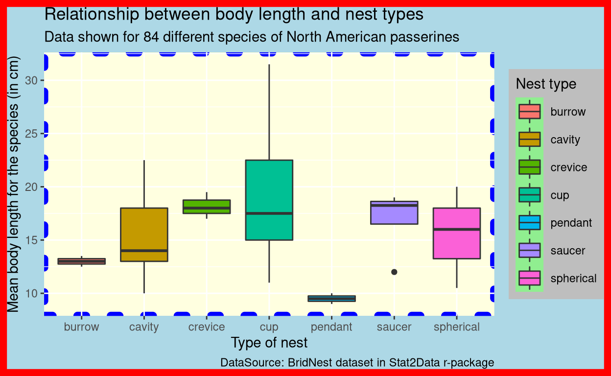
Summary
I hope you are now able to customize a theme of a graph with ease. In this chapter, we learned about different theme elements and how to customize them. We also saw different packages in R which featured ready to use themes. We learned about colour palettes and got introduced to the popular colour packages available R. With that being said, always make sure that your graphs are colour-blind friendly. Have a good day!
Next chapter:
4. Publication ready plots using ggpubr Previous chapter:
2. Customizing graphs in ggplot2
References
H. Wickham. ggplot2: Elegant Graphics for Data Analysis. Springer-Verlag New York, 2016. Read more about ggplot2 here. You can also look at the cheat sheet for all the syntax used in
ggplot2. Also check this out.Ann Cannon, George Cobb, Bradley Hartlaub, Julie Legler, Robin Lock, Thomas Moore, Allan Rossman and Jeffrey Witmer (2019). Stat2Data: Datasets for Stat2. R package version 2.0.0. https://CRAN.R-project.org/package=Stat2Data
Horst AM, Hill AP, Gorman KB (2020). palmerpenguins: Palmer Archipelago (Antarctica) penguin data. R package version 0.1.0. https://allisonhorst.github.io/palmerpenguins/
Jeffrey B. Arnold (2021). ggthemes: Extra Themes, Scales and Geoms for ‘ggplot2’. R package version 4.2.4. https://CRAN.R-project.org/package=ggthemes
Simon Garnier, Noam Ross, Robert Rudis, Antônio P. Camargo, Marco Sciaini, and Cédric Scherer (2021). Rvision - Colorblind-Friendly Color Maps for R. R package version 0.6.2. You can read more here.
Karthik Ram and Hadley Wickham (2018). wesanderson: A Wes Anderson Palette Generator. R package version 0.3.6. https://CRAN.R-project.org/package=wesanderson
Nan Xiao (2018). ggsci: Scientific Journal and Sci-Fi Themed Color Palettes for ‘ggplot2’. R package version 2.9. https://CRAN.R-project.org/package=ggsci
Last updated on
[1] "2022-01-07 22:15:24 IST"